32-2 Induced Magnetic Fields#
Prompts
Explain how a changing electric flux induces a magnetic field. What is the symmetry with Faraday’s law, and why does Maxwell’s law have no minus sign?
What is the capacitor paradox? Ampère’s law says current produces a magnetic field, but between the plates of a charging capacitor there is no conduction current. Why does Ampère’s law alone give contradictory results for different surface choices, and what does Maxwell add to fix it?
To apply the Ampere–Maxwell law, I need to pick a surface bounded by my loop. The law involves both current through that surface and the rate of change of electric flux through it. Does it matter which surface I choose? Walk me through why the result is the same.
Lecture Notes#
Overview#
Faraday (Chap 30): Changing \(\vec{B}\) → induces \(\vec{E}\)
Maxwell: Changing \(\vec{E}\) → induces \(\vec{B}\)
Same structure: Both relate circulation of the induced field to the rate of change of flux
Physical intuition
Electric and magnetic fields are coupled: a changing field of one kind creates the other. This symmetry is central to electromagnetic waves and Maxwell’s equations.
Maxwell’s law of induction#
\(C\): Closed loop — the curve along which we integrate \(\vec{B} \cdot d\vec{s}\)
\(\Sigma\): Any open surface bounded by \(C\) (s.t. \(\partial \Sigma = C\)). \(\Phi_E\vert_\Sigma = \int_\Sigma \vec{E} \cdot d\vec{A}\) is the flux through \(\Sigma\).
Statement: A changing electric flux through \(\Sigma\) induces a magnetic field around \(C\)
Direction: Right-hand rule with \(d\Phi_E/dt\) (no minus sign, unlike Faraday)
Sign convention
Faraday’s law has a minus sign (Lenz’s law: induced \(\vec{E}\) opposes the change).
Maxwell’s law has no minus sign (see Eq. (207)). The opposite sign conventions are crucial: they allow electromagnetic waves to propagate in an oscillatory manner through a negative feedback loop.
Charging capacitor: induced \(\vec{B}\) from changing \(\vec{E}\)#
Setup: Parallel-plate capacitor being charged by constant current \(i\)
Loop \(C\): Circle of radius \(r\) between the plates, concentric with the plates. The same loop \(C\) can bound different surfaces.
Two choices of surface (both have \(\partial \Sigma = C\)):
Surface |
Path |
\(i_{\text{enc}}\) |
\(d\Phi_E/dt\) |
|---|---|---|---|
\(\Sigma_{\text{wire}}\) |
Surface that cuts the wire |
\(\neq 0\) |
\(\sim 0\) |
\(\Sigma_{\text{gap}}\) |
Disk through the gap (avoids the wire) |
\(0\) |
\(\neq 0\) (growing \(\vec{E}\)) |
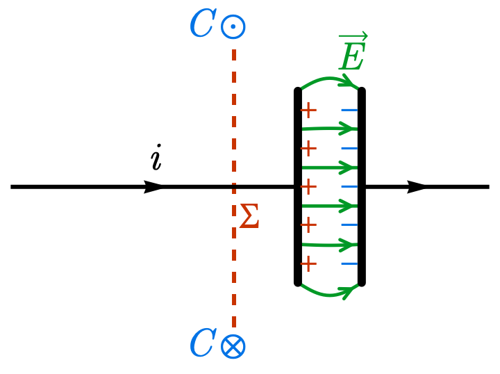
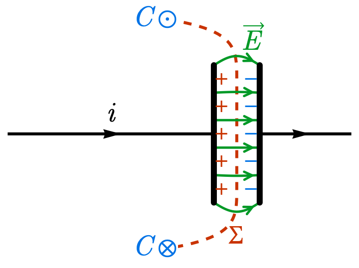
Fig. 20 Two choices of surface \(\Sigma\) bounded by loop \(C\): (a) \(\Sigma_{\text{wire}}\) (cuts wire) — Surface cutting the wire, \(i_{\text{enc}} = i\), conduction current enclosed. (b) \(\Sigma_{\text{gap}}\) (avoids wire) — Surface through the gap, \(i_{\text{enc}} = 0\), \(d\Phi_E/dt \neq 0\).#
Result: \(\vec{B}\) is induced around \(C\) (circular field lines, like a current)
The capacitor paradox
Paradox (Ampere’s law alone): For the same loop \(C\), \(\Sigma_{\text{gap}}\) gives \(i_{\text{enc}} = 0\) (no wire pierces it) while \(\Sigma_{\text{wire}}\) gives \(i_{\text{enc}} = i\). Ampere’s law \(\oint_C \vec{B} \cdot d\vec{s} = \mu_0 i_{\text{enc}}\) would give different values for \(\oint_C \vec{B} \cdot d\vec{s}\) — a contradiction, since the left-hand side is fixed by the actual \(\vec{B}\) field.
Resolution (Ampere–Maxwell law): On \(\Sigma_{\text{gap}}\), \(i_{\text{enc}} = 0\) but \(\mu_0\varepsilon_0\,d\Phi_E/dt\) is non-zero and equals \(\mu_0 i\). On \(\Sigma_{\text{wire}}\), both terms contribute. Both surfaces yield the same \(\oint_C \vec{B} \cdot d\vec{s}\).
Physical intuition: continuity of current
Between the plates there is no conduction current, but \(\vec{E}\) is changing. Maxwell’s term \(\mu_0\varepsilon_0\,d\Phi_E/dt\) acts like a “displacement current” and produces \(\vec{B}\) the same way a real current would. This closes the gap in Ampere’s law.
Ampere’s law vs Maxwell’s law#
Ampere’s law |
Maxwell’s law |
|---|---|
\(\oint_C \vec{B} \cdot d\vec{s} = \mu_0 i_{\text{enc}}\vert_\Sigma\) |
\(\oint_C \vec{B} \cdot d\vec{s} = \mu_0\varepsilon_0 \frac{d\Phi_E}{dt}\big\vert_\Sigma\) |
Current through \(\Sigma\) produces \(\vec{B}\) |
Changing \(\Phi_E\) through \(\Sigma\) produces \(\vec{B}\) |
Steady currents |
Capacitors, time-varying fields |
Ampere–Maxwell law (combined)#
\(C\): Closed loop; \(\Sigma\): open surface with \(\partial \Sigma = C\). Both \(\Phi_E\) and \(i_{\text{enc}}\) are computed on the same \(\Sigma\).
Both sources: \(\vec{B}\) from conduction current through \(\Sigma\) and from changing \(\Phi_E\) through \(\Sigma\)
Wire with steady current: \(d\Phi_E/dt\vert_\Sigma = 0\) → Ampere’s law only
Capacitor gap (no current through \(\Sigma\)): \(i_{\text{enc}}\vert_\Sigma = 0\) → Maxwell’s law only
General method
For any closed loop \(C\):
Choose an open surface \(\Sigma\) with \(\partial \Sigma = C\).
Compute \(i_{\text{enc}}\vert_\Sigma\) (current through \(\Sigma\)) and \(\Phi_E\vert_\Sigma = \int_\Sigma \vec{E} \cdot d\vec{A}\).
Add both contributions.
The result is independent of which \(\Sigma\) you choose. Use symmetry (e.g., circular loops) to simplify.
Summary#
Changing \(\vec{E}\) induces \(\vec{B}\) (Maxwell’s law)
\(\oint_C \vec{B} \cdot d\vec{s} = \mu_0\varepsilon_0\,d\Phi_E/dt\vert_\Sigma\) (no minus sign); \(\Sigma\) is any open surface with \(\partial \Sigma = C\)
Charging capacitor: \(\vec{B}\) between plates from changing \(\vec{E}\) only
Ampere–Maxwell law: \(\vec{B}\) from current and from \(d\Phi_E/dt\)