5.2.3 Applications#

Prompts

What does first-order time-dependent perturbation theory compute in practice, and why can many applications be reduced to transition amplitudes and probabilities?
For a harmonic drive, why does the transition probability develop a resonance profile, and what controls the peak position and spectral width?
Why does the long-time limit lead to Fermi’s golden rule, and what makes the resonance condition \(E_f-E_i=\hbar\omega\) emerge in that limit?
For an adiabatic exponential turn-on, why is the transition profile Lorentzian in detuning, and how does the adiabatic limit connect to the stationary perturbative picture?
In linear response, why is \(\delta\hat{H}=-\hat{\boldsymbol{j}}\cdot\delta\boldsymbol{A}\) the right perturbation for weak electromagnetic driving, and how does this lead to the Kubo view of Hall conductivity?

Lecture Notes#

Overview#

Section 5.2.2 produced the Dyson series for the dressed Green’s function \(\hat{G}(t,t_0)\) (Eq. (195)). This subsection answers the experimentally meaningful question: if a system is prepared in \(\vert i\rangle\) at time \(t_0\), what is the probability to find it in \(\vert f\rangle\) at time \(t\)? The answer is the squared first-order matrix element of \(\hat{G}\), which evaluates differently for different shapes of \(\hat{V}(t)\). Three iconic results follow:

Fermi’s golden rule — sudden harmonic drive in the long-time limit gives a transition rate \(\propto\vert V_{fi}\vert^2\,\delta(E_f-E_i-\hbar\omega)\).
Adiabatic process — exponential ramp gives a Lorentzian in \(\Delta E\) and recovers the time-independent perturbation result (5.1.2) as \(\tau\to\infty\).
Kubo formula — replace the drive by a vector potential and the observable by a current; first-order linear response gives the conductivity, with quantized Hall response on filled Landau levels.

All three share the same one-line input, Eq. (197) below; the differences are entirely in the time profile of \(\hat{V}(t)\).

Transition Probability#

Prepare the system in an eigenstate \(\vert i\rangle\) of \(\hat{H}_0\) at time \(t_0\). After time \(t\), evolution under \(\hat{H}=\hat{H}_0+\hat{V}(t)\) takes it to \(\hat{G}(t,t_0)\vert i\rangle\). The probability to measure \(\vert f\rangle\) is

(196)#\[ \boxed{\; P_{i\to f}(t,t_0)=\bigl\vert\langle f\vert\hat{G}(t,t_0)\vert i\rangle\bigr\vert^2.\;} \]

For \(f\neq i\), the leading nonzero contribution comes from the first-order Dyson term in Eq. (195):

\[ \hat{G}(t,t_0)\simeq \hat{G}_0(t,t_0)-\frac{\mathrm{i}}{\hbar}\!\int_{t_0}^{t}\!\mathrm{d}t_1\,\hat{G}_0(t,t_1)\,\hat{V}(t_1)\,\hat{G}_0(t_1,t_0). \]

Sandwich between \(\langle f\vert\) and \(\vert i\rangle\). Since \(f\neq i\), \(\langle f\vert\hat{G}_0(t,t_0)\vert i\rangle=0\). Insert the spectral form Eq. (193) to extract Bohr phases:

Derivation: phase cancellation in the first-order amplitude

Eigenstate shortcuts give \(\hat{G}_0(t,t_1)\to\mathrm{e}^{-\mathrm{i}E_f(t-t_1)/\hbar}\) on \(\langle f\vert\) and \(\hat{G}_0(t_1,t_0)\vert i\rangle\to\mathrm{e}^{-\mathrm{i}E_i(t_1-t_0)/\hbar}\vert i\rangle\). Hence

\[ \langle f\vert\hat{G}(t,t_0)\vert i\rangle \simeq -\frac{\mathrm{i}}{\hbar}\!\int_{t_0}^{t}\!\mathrm{d}t_1\,\mathrm{e}^{-\mathrm{i}E_f(t-t_1)/\hbar}\,V_{fi}(t_1)\,\mathrm{e}^{-\mathrm{i}E_i(t_1-t_0)/\hbar}, \]

where \(V_{fi}(t_1)\equiv\langle f\vert\hat{V}(t_1)\vert i\rangle\). Collect the \(t_1\)-independent phases:

\[ \langle f\vert\hat{G}(t,t_0)\vert i\rangle \simeq -\frac{\mathrm{i}}{\hbar}\,\mathrm{e}^{-\mathrm{i}E_f t/\hbar}\,\mathrm{e}^{\mathrm{i}E_i t_0/\hbar}\!\int_{t_0}^{t}\!\mathrm{d}t_1\,V_{fi}(t_1)\,\mathrm{e}^{\mathrm{i}\omega_{fi}t_1}, \]

with \(\omega_{fi}\equiv(E_f-E_i)/\hbar\). The leading \(t_1\)-independent phases drop out of \(\vert\cdot\vert^2\).

The transition probability to first order in \(\hat{V}\) is then

(197)#\[ \boxed{\; P_{i\to f}^{(1)}(t,t_0)=\frac{1}{\hbar^2}\left\vert\int_{t_0}^{t}\!\mathrm{d}t_1\,V_{fi}(t_1)\,\mathrm{e}^{\mathrm{i}\omega_{fi}t_1}\right\vert^{2}.\;} \]

where \(\omega_{fi}\equiv(E_f-E_i)/\hbar\) is the Bohr frequency of the \(i\to f\) transition. This is the single time integral that the rest of the lecture evaluates for different time profiles of \(\hat{V}(t)\).

Fermi’s Golden Rule#

Take a sudden harmonic perturbation switched on at \(t_0=0\):

\[\begin{split} \hat{V}(t)=\begin{cases} \hat{V}\,\mathrm{e}^{-\mathrm{i}\omega t}, & t>0,\\[4pt] 0, & t\le 0, \end{cases} \end{split}\]

so \(V_{fi}(t_1)=V_{fi}\,\mathrm{e}^{-\mathrm{i}\omega t_1}\) with \(V_{fi}\equiv\langle f\vert\hat{V}\vert i\rangle\) time-independent. Substituting into Eq. (197):

\[ \int_0^t\!\mathrm{d}t_1\,\mathrm{e}^{\mathrm{i}(\omega_{fi}-\omega)t_1}=\frac{\mathrm{e}^{\mathrm{i}(\omega_{fi}-\omega)t}-1}{\mathrm{i}(\omega_{fi}-\omega)}, \]

and taking the squared modulus:

(198)#\[ \boxed{\; P_{i\to f}^{(1)}(t)=\frac{\vert V_{fi}\vert^{2}}{\hbar^{2}}\left[\frac{\sin\!\bigl((\omega_{fi}-\omega)t/2\bigr)}{(\omega_{fi}-\omega)/2}\right]^{2}.\;} \]

Fig. 24 shows the harmonic drive and its sinc-squared resonance profile.

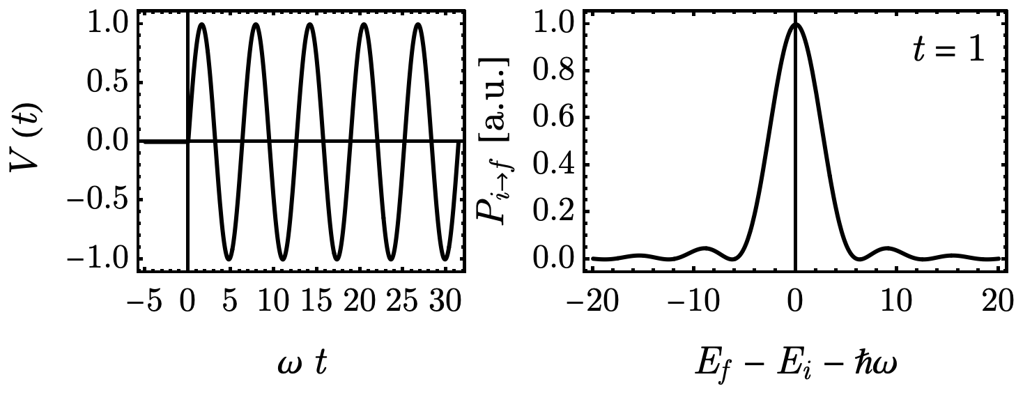
Left panel: a harmonic perturbation V(t) switched on at t=0, oscillating sinusoidally versus omega t. Right panel: the transition probability P from i to f versus the detuning E_f minus E_i minus hbar omega, a sinc-squared curve peaked at zero with decaying side lobes. — Fig. 24 Sudden harmonic drive. **Left:** \(\hat{V}(t)\propto\mathrm{e}^{-\mathrm{i}\omega t}\) switched on at \(t=0\). **Right:** the sinc-squared lineshape Eq. (198) in the detuning \(E_f-E_i-\hbar\omega\), peaked at resonance and narrowing as \(t\) grows toward the golden-rule \(\delta\)-function.#

Derivation: exponential to sinc-squared

Let \(\alpha=(\omega_{fi}-\omega)/2\). Then

\[ \frac{\mathrm{e}^{\mathrm{i}2\alpha t}-1}{2\mathrm{i}\alpha} =\mathrm{e}^{\mathrm{i}\alpha t}\,\frac{\mathrm{e}^{\mathrm{i}\alpha t}-\mathrm{e}^{-\mathrm{i}\alpha t}}{2\mathrm{i}\alpha} =\mathrm{e}^{\mathrm{i}\alpha t}\,\frac{\sin(\alpha t)}{\alpha}, \]

so \(\vert(\mathrm{e}^{\mathrm{i}2\alpha t}-1)/(2\mathrm{i}\alpha)\vert^{2}=\sin^{2}(\alpha t)/\alpha^{2}\).

Properties of the sinc-squared kernel

Setting \(\alpha=(\omega_{fi}-\omega)/2\), the kernel \((\sin\alpha t/\alpha)^{2}\) has

a peak at \(\alpha=0\) (resonance) of height \(t^{2}\),
a width of order \(1/t\),
a total weight \(\int\mathrm{d}\alpha\,(\sin\alpha t/\alpha)^{2}=\pi t\) that grows linearly in \(t\).

The product (peak height)\(\times\)(width)\(\sim t\) is what makes a constant rate emerge after summing over a continuum of final states.

Long-time limit. Use the distribution identity

\[ \lim_{t\to\infty}\frac{1}{t}\left(\frac{\sin\alpha t}{\alpha}\right)^{\!2}=\pi\,\delta(\alpha)=2\pi\,\delta(2\alpha), \]

and define the transition rate \(W_{i\to f}\equiv\lim_{t\to\infty}P_{i\to f}^{(1)}(t)/t\). Then

Fermi’s golden rule

(199)#\[ \boxed{\; W_{i\to f}=\frac{2\pi}{\hbar}\,\vert\langle f\vert\hat{V}\vert i\rangle\vert^{2}\,\delta\!\bigl(E_f-E_i-\hbar\omega\bigr).\;} \]

The delta enforces resonance: the perturbation transfers probability between levels separated by \(\hbar\omega\). For static \(\hat{V}\) (\(\omega=0\)), the resonance is at \(E_f=E_i\).

Continuum of final states

Setup. The system is prepared in the single initial state \(\vert i\rangle\) (fixed by preparation, not a distribution). We compute the total rate at which probability leaves \(\vert i\rangle\), summing the per-channel rate \(W_{i\to f}\) over all final states \(\vert f\rangle\) it can decay into. When the final states form a continuum with density \(\rho(E_f)\) (states per unit energy),

\[ W_{i}=\sum_f W_{i\to f}\;\longrightarrow\;\int\mathrm{d}E_f\,\rho(E_f)\,W_{i\to f}=\frac{2\pi}{\hbar}\,\vert\langle f\vert\hat{V}\vert i\rangle\vert^{2}\,\rho(E_f)\Big\vert_{E_f=E_i+\hbar\omega}. \]

The \(\delta(E_f-E_i-\hbar\omega)\) selects the resonance shell, so it is the density of final states there — and the matrix element evaluated there — that sets the rate. The integral runs over final states because the initial state is fixed; there is no distribution over \(i\) to sum.

“But \(P\to\infty\) as \(t\to\infty\)”

For a transition with \(\omega_{fi}\neq\omega\), the long-time condition means \(t\gg 1/\vert\omega_{fi}-\omega\vert\) — a microscopic time that can still be short compared with the depletion time \(\sim\hbar/\vert V_{fi}\vert\). The rate \(W_{i\to f}=P/t\) is meaningful in perturbation theory whenever \(P\ll 1\). Once \(P\) is no longer small, depletion of \(\vert i\rangle\) must be tracked separately (master equations, self-energy).

Discussion: time–energy resolution

The width \(\sim 2\pi/t\) of the sinc-squared peak is the finite-time energy resolution: a perturbation acting only for time \(t\) cannot distinguish energy differences smaller than \(2\pi\hbar/t\). Strict \(\delta\)-function energy conservation only emerges in the limit \(t\to\infty\). How does this connect to the time–energy uncertainty relation, and what changes if the perturbation is a finite pulse of duration \(T\)?

Adiabatic Process#

Now take an exponential ramp from the infinite past, switched off at \(t=0\), with \(\tau>0\):

\[\begin{split} \hat{V}(t)=\begin{cases} \hat{V}\,\mathrm{e}^{t/\tau}, & t<0,\\[4pt] 0, & t\ge 0, \end{cases} \end{split}\]

System prepared in \(\vert i\rangle\) in the infinite past; ask the transition probability to \(\vert f\rangle\) at \(t=0\). Substitute into Eq. (197) with \(t_0\to-\infty\) and \(t\to 0\):

(200)#\[ \boxed{\; P_{i\to f}=\frac{1}{\hbar^{2}}\left\vert\int_{-\infty}^{0}\!\mathrm{d}t_1\,V_{fi}\,\mathrm{e}^{t_1/\tau}\,\mathrm{e}^{\mathrm{i}\omega_{fi}t_1}\right\vert^{2} =\frac{\vert V_{fi}\vert^{2}}{(E_f-E_i)^{2}+(\hbar/\tau)^{2}}.\;} \]

Fig. 25 shows the exponential ramp and its Lorentzian transition profile.

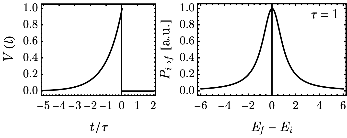
Left panel: a perturbation V(t) growing exponentially as e to the t over tau for t below 0 and cut off at t=0, versus t over tau. Right panel: the transition probability P from i to f versus E_f minus E_i, a Lorentzian peaked at zero with width set by hbar over tau. — Fig. 25 Adiabatic exponential ramp. **Left:** \(\hat{V}(t)\propto\mathrm{e}^{t/\tau}\) for \(t<0\), switched off at \(t=0\). **Right:** the Lorentzian lineshape Eq. (200) in \(\Delta E=E_f-E_i\), centered at zero with width \(\hbar/\tau\).#

Derivation: Lorentzian from the ramp integral

\[ \int_{-\infty}^{0}\!\mathrm{d}t_1\,\mathrm{e}^{(\mathrm{i}\omega_{fi}+1/\tau)t_1} =\Bigl[\frac{\mathrm{e}^{(\mathrm{i}\omega_{fi}+1/\tau)t_1}}{\mathrm{i}\omega_{fi}+1/\tau}\Bigr]_{-\infty}^{0} =\frac{1}{\mathrm{i}\omega_{fi}+1/\tau}, \]

(the lower limit vanishes because \(\tau>0\)). Then

\[ \left\vert\frac{V_{fi}}{\mathrm{i}\omega_{fi}+1/\tau}\right\vert^{2}\!\!/\hbar^{2} =\frac{\vert V_{fi}\vert^{2}}{\hbar^{2}\bigl(\omega_{fi}^{2}+1/\tau^{2}\bigr)} =\frac{\vert V_{fi}\vert^{2}}{(E_f-E_i)^{2}+(\hbar/\tau)^{2}}. \]

The result is a Lorentzian in \(\Delta E=E_f-E_i\), centered at zero with width \(\hbar/\tau\). States closer in energy hybridize more readily; the finite ramp time \(\tau\) sets an energy resolution and regularizes the singularity that would otherwise appear at \(\Delta E=0\).

Adiabatic limit \(\tau\to\infty\): matching to time-independent perturbation theory

As \(\tau\to\infty\) the perturbation is turned on infinitely slowly, and the eigenstate \(\vert i\rangle\) of \(\hat{H}_0\) evolves continuously into the corresponding eigenstate \(\vert i(V)\rangle\) of \(\hat{H}_0+\hat{V}\). To first order in \(\hat{V}\) (cf. 5.1.2),

\[ \vert i(V)\rangle = \vert i\rangle + \sum_{m\neq i}\vert m\rangle\,\frac{V_{mi}}{E_i-E_m}+\cdots, \]

\[ \vert\langle f\vert i(V)\rangle\vert^{2}=\frac{\vert V_{fi}\vert^{2}}{(E_i-E_f)^{2}}, \]

which matches the \(\tau\to\infty\) limit of Eq. (200). Time-dependent perturbation theory falls back to time-independent perturbation theory when the perturbation changes slowly enough.

For any realistic process, \(\tau\) is finite. The Lorentzian width \(\hbar/\tau\) is the uncertainty-principle resolution: the apparent singularity of the energy denominator in time-independent perturbation theory is smoothed out — a genuine physical fact, not an artefact of approximation.

Poll: when does the Lorentzian narrow to the static answer?

The transition probability \(P_{i\to f}\) from an exponential ramp is Eq. (200). As \(\tau\to\infty\) the Lorentzian narrows. Which statement best describes the limit?

(A) \(P_{i\to f}\to 0\) for every fixed \(\Delta E\neq 0\), but the integrated weight is finite and matches the static perturbation result \(\vert V_{fi}/(E_i-E_f)\vert^{2}\) at \(\Delta E\neq 0\).

(B) \(P_{i\to f}\to\infty\) at \(\Delta E=0\) regardless of \(V_{fi}\).

(D) The Lorentzian becomes a Gaussian.

Kubo Formula#

The same first-order machinery applies when the perturbation is a vector potential and the observable is a current. Couple the system to a uniform electric field switched on adiabatically (the same exponential ramp logic as the previous section, with \(\tau^{-1}\to 0^{+}\)):

\[\begin{split} \begin{split} \boldsymbol{E}(t)&=\boldsymbol{E}\,\mathrm{e}^{-\mathrm{i}(\omega+\mathrm{i}0^{+})t},\\ \delta\boldsymbol{A}(t)&=-\frac{\mathrm{i}\boldsymbol{E}}{\omega+\mathrm{i}0^{+}}\,\mathrm{e}^{-\mathrm{i}(\omega+\mathrm{i}0^{+})t},\\ \boldsymbol{E}(t)&=-\partial_t\delta\boldsymbol{A}(t). \end{split} \end{split}\]

Minimal coupling gives the perturbation

(201)#\[ \delta\hat{H}(t)=-\hat{\boldsymbol{j}}\cdot\delta\boldsymbol{A}(t). \]

To match the convention used in 4.3.3 Quantum Hall Effect, we keep the sample area \(A\) explicit (rather than setting \(A=1\)).

Derivation: Kubo formula

Each electron occupies a state \(\vert\alpha\rangle\) that evolves independently under \(\hat{H}_0 + \delta\hat{H}(t)\). We compute the response state-by-state, then sum over occupied states and divide by \(A\) to assemble the macroscopic current density \(\boldsymbol{j}\) via the current-density definition.

Step 1 — First-order response of one occupied state.

Each occupied single-particle state \(\vert\alpha\rangle\) evolves under the interaction-picture operator \(\hat{U}_{\mathcal{I}}(t)\) from §5.2.1. The expectation value of the single-particle current in that state is

\[ \langle\hat{j}_a(t)\rangle_\alpha \equiv \langle\alpha\vert\hat{U}_{\mathcal{I}}^\dagger(t)\,\hat{j}_a^{\mathcal{I}}(t)\,\hat{U}_{\mathcal{I}}(t)\vert\alpha\rangle. \]

Expanding to first order in \(\delta\hat{H}\) gives the standard first-order Kubo identity,

\[ \langle\hat{j}_a(t)\rangle_\alpha = \langle\alpha\vert\hat{j}_a^{\mathcal{I}}(t)\vert\alpha\rangle - \frac{\mathrm{i}}{\hbar}\int_{-\infty}^{t}\!\mathrm{d}t'\,\langle\alpha\vert[\hat{j}_a^{\mathcal{I}}(t),\delta\hat{H}_{\mathcal{I}}(t')]\vert\alpha\rangle, \]

with \(\hat{j}_a^{\mathcal{I}}(t) = \mathrm{e}^{\mathrm{i}\hat{H}_0 t/\hbar}\hat{j}_a\,\mathrm{e}^{-\mathrm{i}\hat{H}_0 t/\hbar}\).

Step 2 — Sum over occupied states; assemble the current density.

Substitute \(\delta\hat{H}_{\mathcal{I}}(t') = -\hat{j}_b^{\mathcal{I}}(t')\,\delta A_b(t')\), sum over occupied states, and divide by \(A\). The zeroth-order term \(\sum_{\alpha\in\mathrm{occ}}\langle\alpha\vert\hat{j}_a\vert\alpha\rangle = 0\) vanishes (no current without a driving field), leaving

\[ j_a(t) = \frac{\mathrm{i}}{\hbar A}\!\int_{-\infty}^{t}\!\mathrm{d}t'\,\delta A_b(t')\sum_{\alpha\in\mathrm{occ}}\langle\alpha\vert[\hat{j}_a^{\mathcal{I}}(t),\hat{j}_b^{\mathcal{I}}(t')]\vert\alpha\rangle. \]

Step 3 — Substitute the harmonic field.

Using \(\delta A_b(t') = (-\mathrm{i}E_b/(\omega+\mathrm{i}0^+))\,\mathrm{e}^{-\mathrm{i}(\omega+\mathrm{i}0^+)t'}\) and the change of variable \(\tau = t-t'\) (with time-translation invariance of the unperturbed system), the result \(j_a(t) = \sigma_{ab}(\omega)\,E_b\,\mathrm{e}^{-\mathrm{i}(\omega+\mathrm{i}0^+)t}\) defines

\[ \sigma_{ab}(\omega) = -\frac{1}{\hbar(\omega+\mathrm{i}0^+) A}\int_0^{\infty}\!\mathrm{d}\tau\,\mathrm{e}^{\mathrm{i}(\omega+\mathrm{i}0^+)\tau}\sum_{\alpha\in\mathrm{occ}}\langle\alpha\vert[\hat{j}_a^{\mathcal{I}}(\tau),\hat{j}_b^{\mathcal{I}}(0)]\vert\alpha\rangle. \]

Step 4 — Insert eigenbasis and evaluate the time integral.

Insert \(\sum_\gamma\vert\gamma\rangle\langle\gamma\vert\) between the two single-particle current operators and use the matrix-element identity \(\langle\alpha\vert\hat{j}_a^{\mathcal{I}}(\tau)\vert\gamma\rangle = \mathrm{e}^{-\mathrm{i}\omega_{\gamma\alpha}\tau}\,\langle\alpha\vert\hat{j}_a\vert\gamma\rangle\) on each \(\langle\alpha\vert\cdots\vert\alpha\rangle\) matrix element (with \(\omega_{\gamma\alpha} = (E_\gamma-E_\alpha)/\hbar\)),

\[ \sum_{\alpha\in\mathrm{occ}}\langle\alpha\vert[\hat{j}_a^{\mathcal{I}}(\tau),\hat{j}_b^{\mathcal{I}}(0)]\vert\alpha\rangle = \sum_{\alpha\in\mathrm{occ}}\sum_\gamma\Big(j^a_{\alpha\gamma}j^b_{\gamma\alpha}\,\mathrm{e}^{-\mathrm{i}\omega_{\gamma\alpha}\tau} - j^b_{\alpha\gamma}j^a_{\gamma\alpha}\,\mathrm{e}^{\mathrm{i}\omega_{\gamma\alpha}\tau}\Big), \]

with \(j^a_{\alpha\gamma} \equiv \langle\alpha\vert\hat{j}_a\vert\gamma\rangle\) a single-particle matrix element. The \(\tau\) integral gives \(\int_0^\infty\!\mathrm{d}\tau\,\mathrm{e}^{\mathrm{i}(\omega+\mathrm{i}0^+ \pm\omega_{\gamma\alpha})\tau} = \mathrm{i}/(\omega+\mathrm{i}0^+\pm\omega_{\gamma\alpha})\).

Step 5 — DC limit.

For \(\gamma = \alpha\) (intra-band), the integrand is finite but the prefactor \(1/\omega\) produces a pole — the Drude weight, which is absent for a gapped insulator and irrelevant to the antisymmetric Hall part. For \(\gamma\neq\alpha\) (inter-band), expand \(1/(\omega\pm\omega_{\gamma\alpha}) = \pm 1/\omega_{\gamma\alpha} - \omega/\omega_{\gamma\alpha}^2 + O(\omega^2)\). The \(\pm 1/\omega_{\gamma\alpha}\) piece, divided by \(\omega\), gives the symmetric (longitudinal) divergence that cancels in clean systems with current conservation. The \(-\omega/\omega_{\gamma\alpha}^2\) piece gives a finite antisymmetric contribution. Restricting \(\gamma\notin\mathrm{occ}\) — terms with \(\gamma\in\mathrm{occ}\) pair-cancel because both \(\alpha\) and \(\gamma\) run over the occupied set — yields

\[ \sigma_{xy} = \frac{\mathrm{i}\hbar}{A}\sum_{\alpha\in\mathrm{occ}}\sum_{\beta\notin\mathrm{occ}}\frac{\langle\alpha\vert\hat{j}_x\vert\beta\rangle\langle\beta\vert\hat{j}_y\vert\alpha\rangle - \langle\alpha\vert\hat{j}_y\vert\beta\rangle\langle\beta\vert\hat{j}_x\vert\alpha\rangle}{(E_\beta-E_\alpha)^2}, \]

the Kubo formula above. All matrix elements are single-particle (\(\hat{j}\)); the \(1/A\) traces back to using current density (current per unit area).

Substitute into Eq. (197) and compute the first-order response of the current \(\langle\hat{\boldsymbol{j}}\rangle\) on a filled-band ground state at \(T=0\). The result is the Hall conductivity:

Kubo formula (zero temperature)

(202)#\[ \sigma_{xy}=\frac{\mathrm{i}\hbar}{A} \sum_{\alpha\in\mathrm{occ}}\sum_{\beta\notin\mathrm{occ}} \frac{\langle\alpha\vert\hat{j}_x\vert\beta\rangle\langle\beta\vert\hat{j}_y\vert\alpha\rangle- \langle\alpha\vert\hat{j}_y\vert\beta\rangle\langle\beta\vert\hat{j}_x\vert\alpha\rangle} {(E_\beta-E_\alpha)^{2}}. \]

A transport coefficient written entirely in terms of virtual transitions between occupied \(\vert\alpha\rangle\) and empty \(\vert\beta\rangle\) states. The energy-denominator structure mirrors the time-independent perturbation theory of 5.1.2, now for a many-body filled ground state.

Evaluating Eq. (202) for \(\nu\) completely filled Landau levels gives the exact integer Hall quantization

\[ \sigma_{xy}=\nu\,\frac{e^2}{h}, \]

connecting first-order perturbation theory to a topologically protected observable (details in §4.3.3).

Summary#

Transition probability: \(P_{i\to f}=\vert\langle f\vert\hat{G}(t,t_0)\vert i\rangle\vert^{2}\); first order in \(\hat{V}\) collapses to a single time integral involving the matrix element \(V_{fi}(t_1)\) and the Bohr phase \(\mathrm{e}^{\mathrm{i}\omega_{fi}t_1}\).
Fermi’s golden rule: sudden harmonic drive \(\hat{V}\mathrm{e}^{-\mathrm{i}\omega t}\) produces a sinc-squared resonance whose long-time limit is a rate \(W_{i\to f}=\frac{2\pi}{\hbar}\vert V_{fi}\vert^{2}\,\delta(E_f-E_i-\hbar\omega)\).
Adiabatic process: exponential ramp \(\hat{V}\mathrm{e}^{t/\tau}\) produces a Lorentzian in \(\Delta E\) of width \(\hbar/\tau\); the \(\tau\to\infty\) limit recovers the energy-denominator language of 5.1.2.
Kubo formula: the same first-order machinery applied to \(\delta\hat{H}=-\hat{\boldsymbol{j}}\cdot\delta\boldsymbol{A}\) gives the Hall conductivity; integer-filled Landau levels yield the topological quantization \(\sigma_{xy}=\nu e^2/h\).

Homework#

1. Phase cancellation. Verify in detail the cancellation of the overall \(\mathrm{e}^{-\mathrm{i}E_f t/\hbar}\mathrm{e}^{\mathrm{i}E_i t_0/\hbar}\) phase in the first-order amplitude \(\langle f\vert\hat{G}(t,t_0)\vert i\rangle\), and conclude that \(P_{i\to f}^{(1)}\) depends only on \(V_{fi}(t_1)\mathrm{e}^{\mathrm{i}\omega_{fi}t_1}\). Why is this cancellation expected on general grounds?

2. Sinc-squared properties. From \(P_{i\to f}^{(1)}(t)=\frac{\vert V_{fi}\vert^2}{\hbar^2}\bigl[\sin((\omega_{fi}-\omega)t/2)/((\omega_{fi}-\omega)/2)\bigr]^2\) with \(\alpha=(\omega_{fi}-\omega)/2\), derive each of the following:

(a) Peak height \(P^{(1)}\vert_{\alpha=0}=\vert V_{fi}\vert^{2}t^{2}/\hbar^{2}\).

(b) First zero at \(\alpha t=\pi\), i.e. width \(\Delta\alpha\sim\pi/t\).

Explain why (a)\(\times\)(b)\(\sim\)(c) is the algebraic origin of a constant rate in the long-time limit.

3. Sinc-to-delta. Prove the distributional identity

\[ \lim_{t\to\infty}\frac{1}{t}\left(\frac{\sin\alpha t}{\alpha}\right)^{\!2}=\pi\,\delta(\alpha). \]

Hint: act on a smooth test function \(g(\alpha)\) and use the change of variable \(u=\alpha t\) together with \(\int_{-\infty}^{\infty}(\sin u/u)^{2}\,\mathrm{d}u=\pi\).

4. Density of states. For free particles in three dimensions in a box of volume \(V\),

(a) Show that the density of states is \(\rho(E)=\dfrac{V m}{2\pi^{2}\hbar^{3}}\sqrt{2mE}\).

(b) Use Fermi’s golden rule with this \(\rho\) to express \(W_i\) in terms of \(\vert V_{fi}\vert^{2}\), the drive frequency \(\omega\), and the initial energy \(E_i\). How does \(W_i\) scale with \(E_i\) at fixed \(\vert V_{fi}\vert\)?

5. Adiabatic ramp Lorentzian. Derive \(P_{i\to f}=\frac{\vert V_{fi}\vert^2}{(E_f-E_i)^2+(\hbar/\tau)^2}\) step by step, starting from \(\hat{V}(t)=\hat{V}\mathrm{e}^{t/\tau}\) for \(t<0\). State the FWHM in \(\omega_{fi}\) and in \(\Delta E=E_f-E_i\), and sketch the lineshape.

6. Adiabatic to static perturbation. Take the \(\tau\to\infty\) limit of \(P_{i\to f}=\frac{\vert V_{fi}\vert^2}{(E_f-E_i)^2+(\hbar/\tau)^2}\) for fixed \(\Delta E\neq 0\), and compare with \(\vert\langle f\vert i(V)\rangle\vert^{2}\) from non-degenerate perturbation theory (5.1.2). Explain physically why the two answers must agree.

★ 7. Three-level Raman (long-time limit). Continue the setup from HW 5.2.2.8: \(\hat{H}_0=\Delta\vert 3\rangle\langle 3\vert\) with \(E_1=E_2=0\), \(E_3=\Delta>0\), and \(\hat{V}(t)=\lambda(t)[(\vert 1\rangle+\vert 2\rangle)\langle 3\vert+\mathrm{h.c.}]\) with \(\lambda(t)=\lambda_0\cos(\omega t)\).

(a) Starting from the second-order amplitude \(\langle 2\vert\hat{G}(t,0)\vert 1\rangle\) obtained in HW 5.2.2.8, evaluate the double time integral in the long-time limit \(\omega^{-1},\Delta^{-1}\ll t\ll\lambda_0^{-1}\). Identify which of the four oscillating terms contribute (those whose total exponent vanishes) and show

\[ \langle 2\vert\hat{G}(t,0)\vert 1\rangle\approx\frac{\mathrm{i}\,\lambda_0^{2}\,t}{2}\,\frac{\Delta}{\Delta^{2}-\omega^{2}}. \]

(b) Compute \(P_{1\to 2}(t)=\vert\langle 2\vert\hat{G}(t,0)\vert 1\rangle\vert^{2}\) and identify the time scaling and the frequency dependence on \(\omega/\Delta\).

(c) Explain physically why the result is resonantly enhanced near \(\omega/\Delta=1\) and why the time scaling is \(t^{2}\) rather than \(t\) (compare to Fermi’s golden rule).

(d) Near-resonance limit and the rotating wave approximation. Set \(\omega \approx \Delta\) (close to but not exactly at single-photon resonance) and re-evaluate the second-order amplitude under the rotating wave approximation (RWA): of the four oscillating terms identified in (a), keep only the one whose two exponent frequencies are both slow in the limit \(\omega \to \Delta\), and drop the other three as fast-oscillating. Show that the RWA amplitude is

\[ \langle 2\vert\hat{G}(t,0)\vert 1\rangle \approx \frac{\mathrm{i}\,\lambda_0^{2}\,t}{4(\Delta - \omega)}, \]

and verify that this agrees with the full off-resonant result of (a) in the near-resonant limit \(\vert\Delta - \omega\vert \ll \Delta + \omega\).

8. Minimal Kubo exercise. Take a two-level toy with \(\hat{H}_0=-\frac{1}{2}\hbar\omega_0\hat{Z}\), occupied \(\vert 0\rangle\), empty \(\vert 1\rangle\), and current operators \(\hat{j}_x=\hat{X}\), \(\hat{j}_y=\hat{Y}\) (without charge or geometric prefactors).

(a) Compute the four matrix elements entering the Kubo numerator.

(b) Evaluate

\[ \sigma_{xy}=\mathrm{i}\hbar\, \frac{\langle 0\vert\hat{j}_x\vert 1\rangle\langle 1\vert\hat{j}_y\vert 0\rangle-\langle 0\vert\hat{j}_y\vert 1\rangle\langle 1\vert\hat{j}_x\vert 0\rangle}{(E_1-E_0)^{2}}. \]

(c) Replace \(\hat{j}_y\to\hat{X}\) and show that \(\sigma_{xy}\) vanishes — i.e. why a Hall response requires non-commuting current operators.