2.2.1 Angular Momentum Algebra#
Prompts
What are the fundamental commutation relations for angular momentum, and how do they encode the geometry of 3D rotations?
Define the Casimir operator \(\hat{J}^2\) and explain why it commutes with all components of \(\hat{\boldsymbol{J}}\). Why does this allow simultaneous eigenstates \(\vert j, m\rangle\)?
How do the ladder operators \(\hat{J}_\pm\) connect eigenstates with different \(m\)? What is the physical meaning of their normalization coefficients?
Why does angular momentum quantization (\(j = 0, \frac{1}{2}, 1, \ldots\)) follow purely from the commutation algebra? What does this reveal about the power of symmetry?
Lecture Notes#
Overview#
In Chapter 1, we studied a single qubit — the spin-1/2 system with two eigenstates. This raises a natural question: what about higher spin? What constrains the possible values of angular momentum, and how do they arise?
The answer is remarkable: angular momentum quantization follows entirely from commutation relations, without solving any differential equation. All forms of angular momentum — orbital (\(\boldsymbol{L} = \boldsymbol{r} \times \boldsymbol{p}\)), spin (\(\boldsymbol{S}\)), and total (\(\boldsymbol{J} = \boldsymbol{L} + \boldsymbol{S}\)) — satisfy the same algebra. This algebra is the Lie algebra of SU(2), the group of rotations we met in §1.3.3. The physical content is simple: rotations in 3D do not commute, and angular momentum operators are their generators.
Angular Momentum Algebra#
Defining Relation
The three components of any angular momentum operator \(\hat{\boldsymbol{J}}=(\hat J_x,\hat J_y,\hat J_z)\) satisfy
Explicitly,
For orbital angular momentum these follow from \([\hat r_i,\hat p_j]=\mathrm{i}\hbar\delta_{ij}\); for spin they are postulated as the rotation-generator algebra.
Derivation: Orbital Angular Momentum Commutators
Using \(\hat L_i=\epsilon_{imn}\hat r_m\hat p_n\) and the canonical commutators \([\hat r_a,\hat p_b]=\mathrm{i}\hbar\delta_{ab}\), \([\hat r_a,\hat r_b]=[\hat p_a,\hat p_b]=0\):
Using \(\epsilon_{abc}\epsilon_{ade}=\delta_{bd}\delta_{ce}-\delta_{be}\delta_{cd}\) gives
\(\checkmark\)
Casimir Operator.
Casimir Operator
The total angular momentum squared
commutes with every component:
Derivation: \([\hat J^2,\hat J_z]=0\)
Using \([\hat A^2,\hat B]=\hat A[\hat A,\hat B]+[\hat A,\hat B]\hat A\):
which cancel exactly.
Ladder Operators.
Ladder Operators
Define
They satisfy
Derivation: Ladder Operator Commutation Relations
From \(\hat J_\pm=\hat J_x\pm\mathrm{i}\hat J_y\) and \([\hat J_i,\hat J_j]=\mathrm{i}\hbar\epsilon_{ijk}\hat J_k\):
And by linearity,
These commutation relations imply two useful operator identities:
Derivation: Ladder Product Identities
From
we get
Using \([\hat J_+,\hat J_-]=2\hbar\hat J_z\),
Solving these two equations gives (40).
Angular Momentum Representation Theory#
Because \([\hat J^2,\hat J_z]=0\), we can choose simultaneous eigenstates and build irreducible multiplets algebraically.
Common Eigenstates of \(\hat J^2\) and \(\hat J_z\).
Simultaneous Eigenstates
Let \(\vert j,m\rangle\) satisfy
At this stage, \(j,m\in\mathbb{R}\) are labels; quantization is derived below.
Ladder Operator Action.
Ladder Action on \(\vert j,m\rangle\)
So \(\hat J_+\) raises \(m\) by one and \(\hat J_-\) lowers \(m\) by one.
Derivation: Ladder-Action Coefficients
From \([\hat J_z,\hat J_\pm]=\pm\hbar\hat J_\pm\) and \([\hat J^2,\hat J_\pm]=0\), the states \(\hat J_\pm\vert j,m\rangle\) lie in the same \(j\) multiplet with \(m\to m\pm1\).
For normalization, use (40):
Taking square roots yields (42).
Angular Momentum Quantization.
Quantization Rules
For each \(j\), the multiplet dimension is \(2j+1\).
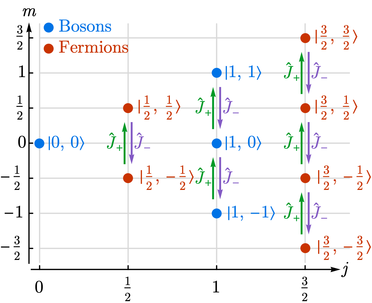
Fig. 3 States \(\vert j,m\rangle\) form vertical ladders in \(m\) for fixed \(j\); \(\hat J_+\) (green) and \(\hat J_-\) (purple) connect adjacent levels. Integer \(j\) (blue) and half-integer \(j\) (red) both satisfy the algebra.#
Proof: Quantum bootstrap argument
The quantum bootstrap is an algebraic method: constrain quantum numbers by positivity of norms. For any operator \(\hat A\) and state \(\vert\psi\rangle\),
Applied to angular momentum, this principle fixes the allowed values of \(j\) and \(m\).
From (41), take simultaneous eigenstates \(\vert j,m\rangle\) of \(\hat J^2\) and \(\hat J_z\).
(1) Positivity constraints. Apply positivity to \(\hat A=\hat J_+\) and \(\hat A=\hat J_-\) on \(\vert j,m\rangle\):
Using (42), these become
So \(m\) is bounded: \(-j\le m\le j\).
(2) Ladder unit-step structure. From \([\hat J_z,\hat J_\pm]=\pm\hbar\hat J_\pm\), each ladder action changes \(m\) by exactly one unit. Therefore all \(m\) values in one multiplet differ by integers.
(3) Finite-dimensional irreducibility. In a finite-dimensional irrep, the ladder must terminate at top and bottom states:
By (42), vanishing coefficients imply
Hence the ladder runs
with \(N=2j+1\) states.
Since \(N\in\mathbb N\), we must have \(2j\in\mathbb N_0\). Therefore
So quantization follows from algebra + positivity + finite-dimensional irreducibility.
Integer vs. half-integer: Orbital angular momentum (\(\hat{\boldsymbol{L}}=\hat{\boldsymbol{r}}\times\hat{\boldsymbol{p}}\)) gives only integer \(\ell\) from single-valued wavefunctions, while spin admits half-integer \(j\).
Matrix Representations.
For fixed \(j\), the operators act on a \((2j+1)\)-dimensional space.
Spin-1/2: Pauli Matrices
For \(j=1/2\):
Spin-1: 3\(\times\)3 Matrices
For \(j=1\):
Discussion: integer vs half-integer angular momentum
Why do orbital and spin angular momentum components differ in their allowed quantum numbers? Orbital angular momentum must have integer \(\ell\) to ensure single-valued wavefunctions in physical space, while spin can have half-integer \(j\). Yet both satisfy the exact same commutation algebra \([\hat{J}_i, \hat{J}_j] = \mathrm{i}\hbar\epsilon_{ijk}\hat{J}_k\). Does this mean the algebra alone cannot distinguish integer from half-integer representations? What is the fundamental reason—is it topology, boundary conditions, or something deeper about the nature of rotation in quantum mechanics?
Poll: Ladder operator eigenvalue shift
Angular momentum operators satisfy \([\hat{J}_x, \hat{J}_y] = \mathrm{i}\hbar\hat{J}_z\). The raising operator is \(\hat{J}_+ = \hat{J}_x + \mathrm{i}\hat{J}_y\). If \(\hat{J}_z\vert j, m\rangle = \hbar m\vert j, m\rangle\), what is \(\hat{J}_z(\hat{J}_+\vert j, m\rangle)\) proportional to?
(A) \(\hat{J}_+\vert j, m\rangle\) with eigenvalue \(\hbar m\) (unchanged).
(B) \(\hat{J}_+\vert j, m\rangle\) with eigenvalue \(\hbar(m+1)\) (raised by 1).
(C) Zero (raising operators are orthogonal to Z eigenstates).
(D) \((\hat{J}_+)^2\vert j, m\rangle\) (squared).
Summary#
All angular momenta satisfy the same commutation relations \([\hat{J}_i, \hat{J}_j] = \mathrm{i}\hbar\epsilon_{ijk}\hat{J}_k\) — the Lie algebra \(\mathfrak{su}(2)\).
The Casimir operator \(\hat{J}^2\) commutes with all components, enabling simultaneous eigenstates \(\vert j, m\rangle\).
Quantization (\(j = 0, \frac{1}{2}, 1, \ldots\); \(m = -j, \ldots, j\)) follows from algebra alone.
Ladder operators \(\hat{J}_\pm\) shift \(m\) by \(\pm 1\) with known normalization.
Representations: spin-1/2 recovers Pauli matrices; spin-1 gives \(3\times 3\) matrices; general \(j\) gives \((2j+1)\)-dimensional irreducible representations.
See Also
1.1.3 Hermitian Operators: Self-adjoint observables and spectral notions reused for \(\hat{J}^2,\hat{J}_z\).
2.2.2 Spin Representations: From \(su(2)\) commutation relations to spin-\(j\) representations and ladder operators.
2.2.3 Addition of Angular Momenta: Tensoring representations, Clebsch–Gordan series, and coupled bases.
Homework#
1. Spin-1 verification of the angular-momentum algebra. The lecture states that the commutation relations \([\hat J_i,\hat J_j] = \mathrm{i}\hbar\epsilon_{ijk}\hat J_k\) hold for any representation. The spin-1/2 case follows from the Pauli commutators (1.1.3). Here, verify the relation directly for the spin-1 representation, in the basis \(\{\vert 1,+1\rangle, \vert 1,0\rangle, \vert 1,-1\rangle\}\) where \(\hat J_z = \hbar\,\mathrm{diag}(1, 0, -1)\) and
(a) Compute \([\hat J_x, \hat J_y]\) by matrix multiplication and verify it equals \(\mathrm{i}\hbar\hat J_z\).
(b) Compute \(\hat J^2 = \hat J_x^2 + \hat J_y^2 + \hat J_z^2\) explicitly and confirm \(\hat J^2 = 2\hbar^2\hat I = \hbar^2 \cdot 1\cdot(1+1)\hat I\), i.e. the Casimir eigenvalue \(j(j+1) = 2\) for \(j = 1\).
(c) Compare with the spin-1/2 case from 1.1.3 (where \(\hat J^2 = \frac{3}{4}\hbar^2\hat I\)). State the general pattern: the Casimir eigenvalue is \(j(j+1)\hbar^2\) for every spin-\(j\) multiplet, set by \(\hat J^2\) alone.
2. j=3/2 multiplet by repeated lowering. Start from the stretched state \(\vert 3/2, 3/2\rangle\) and apply the lowering operator \(\hat J_-\) repeatedly to construct all four states of the spin-\(\tfrac{3}{2}\) multiplet.
(a) Verify that \(\hat J_+\vert 3/2, 3/2\rangle = 0\) using the ladder formula \(\hat J_+\vert j,m\rangle = \hbar\sqrt{(j-m)(j+m+1)}\vert j, m+1\rangle\).
(b) Compute \(\hat J_-\vert 3/2, m\rangle\) for \(m = 3/2, 1/2, -1/2, -3/2\), using \(\hat J_-\vert j,m\rangle = \hbar\sqrt{(j+m)(j-m+1)}\vert j, m-1\rangle\). State the coefficient in each step.
(c) Verify that \(\hat J_-\vert 3/2, -3/2\rangle = 0\) — the multiplet terminates at the bottom rung.
(d) The four states \(\{\vert 3/2, 3/2\rangle, \vert 3/2, 1/2\rangle, \vert 3/2, -1/2\rangle, \vert 3/2, -3/2\rangle\}\) form a \(4\)-dimensional representation. Argue from this construction that the dimension of a spin-\(j\) multiplet is \(2j+1\).
3. Ladder formula via Schwinger bosons. Recall the Schwinger boson construction from 2.1.3 Problem 10: spin operators \(\hat S_+ = \hat a^\dagger\hat b\), \(\hat S_- = \hat b^\dagger\hat a\), \(\hat S_z = \tfrac{1}{2}(\hat a^\dagger\hat a - \hat b^\dagger\hat b)\), with the Fock state \(\vert n_a, n_b\rangle\) identified with \(\vert s, m\rangle\) via \(s = (n_a + n_b)/2\) and \(m = (n_a - n_b)/2\). Use the bosonic algebra to derive the angular-momentum ladder formula.
(a) Express \(n_a\) and \(n_b\) in terms of \(s\) and \(m\).
(b) Apply \(\hat S_+ = \hat a^\dagger\hat b\) to \(\vert n_a, n_b\rangle\) and read off the coefficient using \(\hat a^\dagger\vert n_a\rangle = \sqrt{n_a+1}\vert n_a+1\rangle\) and \(\hat b\vert n_b\rangle = \sqrt{n_b}\vert n_b-1\rangle\). Show that
reproducing the lecture’s ladder formula (in units \(\hbar = 1\)).
(c) Argue that this derivation makes the ladder coefficient \(\sqrt{(s-m)(s+m+1)}\) automatic — it emerges directly from the bosonic normalisation factors \(\sqrt{n}\), with no separate calculation needed. Contrast with the standard approach (lecture), which derives the same coefficient from \(\hat J_+\hat J_- = \hat J^2 - \hat J_z^2 + \hbar\hat J_z\).
4. Ladder action: termination and verification. Use \(\hat J_+\vert j, m\rangle = \hbar\sqrt{(j-m)(j+m+1)}\,\vert j, m+1\rangle\) to explain why \(\hat J_+\vert 1,1\rangle = 0\). Then compute \(\hat J_-\vert 1, 0\rangle\) from the lowering formula and verify the result using the spin-1 matrix representation from Problem 1.
5. Transverse variance on an angular-momentum eigenstate. Compute \(\langle\hat J_x\rangle\), \(\langle\hat J_x^2\rangle\), and the variance \((\Delta\hat J_x)^2\) on a state \(\vert j, m\rangle\).
(a) Express \(\hat J_x = \tfrac{1}{2}(\hat J_+ + \hat J_-)\) and use it to compute \(\langle\hat J_x\rangle = \langle j, m\vert\hat J_x\vert j, m\rangle\). Explain in one sentence why the result is zero.
(b) Use the lecture’s ladder product identity \(\hat J_+\hat J_- + \hat J_-\hat J_+ = 2(\hat J^2 - \hat J_z^2)\) to compute \(\hat J_x^2 + \hat J_y^2 = \tfrac{1}{2}(\hat J_+\hat J_- + \hat J_-\hat J_+) = \hat J^2 - \hat J_z^2\). Conclude
(c) By the symmetry of the algebra under \(x \leftrightarrow y\) on a \(\hat J_z\)-eigenstate, \(\langle\hat J_x^2\rangle = \langle\hat J_y^2\rangle\). Conclude
(d) Identify the limiting values: at the stretched state \(m = \pm j\), \((\Delta\hat J_x)^2 = \hbar^2 j/2\) — not zero, even though the state is a \(\hat J_z\) eigenstate. Explain physically why even the most “extreme” \(\hat J_z\) eigenstate has some transverse uncertainty — the quantum AM vector cannot be perfectly aligned with \(\boldsymbol{e}_z\).
6. Robertson uncertainty for angular momentum. Apply the Robertson uncertainty relation from 1.2.2 to the pair \((\hat J_x, \hat J_y)\) on a state \(\vert j, m\rangle\).
(a) Using \([\hat J_x, \hat J_y] = \mathrm{i}\hbar\hat J_z\), write down the Robertson bound \(\Delta\hat J_x\cdot\Delta\hat J_y \geq \tfrac{1}{2}\vert\langle[\hat J_x, \hat J_y]\rangle\vert\).
(b) Evaluate both sides on the stretched state \(\vert j, j\rangle\). Use the variance from Problem 5 and the fact that \(\langle\hat J_z\rangle_{\vert j, j\rangle} = \hbar j\).
(c) Show that the Robertson inequality is saturated on the stretched state. Why is this the angular-momentum analogue of the minimum-uncertainty state \(\vert 0\rangle\) for \((\hat X, \hat Z)\) from 1.2.2 Problem 6?
(d) Compute the ratio \(\Delta\hat J_x/\langle\hat J_z\rangle\) on the stretched state and show that in the classical limit \(j \to \infty\), this ratio vanishes as \(1/\sqrt j\). The angular momentum becomes a sharp 3-vector in the classical limit, recovering the macroscopic notion of AM.
7. Vector model and the tilt angle. The state \(\vert j, m\rangle\) has \(\langle\hat J^2\rangle = \hbar^2 j(j+1)\), \(\langle\hat J_z\rangle = \hbar m\), and \(\langle\hat J_x\rangle = \langle\hat J_y\rangle = 0\). The vector model pictures the angular momentum as a classical 3-vector of length \(\vert\boldsymbol J\vert = \hbar\sqrt{j(j+1)}\) with \(z\)-component \(J_z = \hbar m\).
(a) Show that the angle \(\theta\) between \(\boldsymbol J\) and the \(z\)-axis satisfies
(b) For the stretched state \(\vert j, j\rangle\), find the minimum tilt angle \(\theta_{\min}\) in terms of \(j\), and evaluate it for \(j = 1/2\), \(j = 1\), and \(j = 100\).
(c) The quantum AM cannot be exactly aligned with \(\boldsymbol{e}_z\): even the stretched state has \(\theta_{\min} > 0\). Use Problem 5 to compute the transverse magnitude \(\sqrt{\langle\hat J_x^2 + \hat J_y^2\rangle} = \hbar\sqrt{j(j+1) - m^2}\) and identify it with the radius of a precession circle in the vector model.
(d) Compare with the classical prediction: for a classical AM vector of length \(\vert\boldsymbol J\vert\) tilted at angle \(\theta\), the transverse projection is \(\vert\boldsymbol J\vert\sin\theta\). Verify that the quantum result \(\hbar\sqrt{j(j+1) - m^2}\) equals \(\vert\boldsymbol J\vert\sin\theta\) using the value of \(\cos\theta\) from (a).
★ 8. Quantum bootstrap. Two operators \(\hat{\alpha}\) and \(\hat{\beta}\) satisfy the algebraic relations
where \([\hat{A}, \hat{B}] = \hat{A}\hat{B} - \hat{B}\hat{A}\) is the commutator, \(\{\hat{A}, \hat{B}\} = \hat{A}\hat{B} + \hat{B}\hat{A}\) is the anticommutator, and \(\hat{I}\) is the identity operator.
(a) Show that \(\hat{\beta}\) is Hermitian.
(b) Express \(\hat{\alpha}^\dagger\hat{\alpha}\) and \(\hat{\alpha}\hat{\alpha}^\dagger\) separately as linear combinations of \(\hat{\beta}\) and \(\hat{I}\).
(c) Show that \((\hat{\alpha}^\dagger)^2 \hat{\alpha}^2 = \hat{\beta}^2 - \hat{I}\) by expressing the left-hand side in terms of \(\hat{\beta}\). Using the positivity conditions \(\hat{\alpha}^\dagger\hat{\alpha} \geq 0\), \(\hat{\alpha}\hat{\alpha}^\dagger \geq 0\), and \((\hat{\alpha}^\dagger)^2\hat{\alpha}^2 \geq 0\), determine the feasible eigenvalues of \(\hat{\beta}\).
(d) Identify the angular momentum operators that \(\hat{\alpha}\) and \(\hat{\beta}\) correspond to (with \(\hbar = 1\)). What spin representation does this algebra describe? Write the \(2\times 2\) matrix representations of \(\hat{\alpha}\) and \(\hat{\beta}\) in the eigenbasis of \(\hat{\beta}\).