1.2.1 Measurement Postulate#

Prompts

State the three parts of the measurement postulate. For each part, explain why it must be true for measurement to connect theory to experiment.
The Born rule says the probability of outcome \(\lambda_i\) is \(\vert\langle\psi_i\vert\psi\rangle\vert^2\). Why do we square the inner product instead of just taking the inner product itself or its absolute value?
After measuring observable \(\hat{O}\) and obtaining outcome \(\lambda_i\), the state collapses to the eigenstate \(\vert\psi_i\rangle\). Is this a physically real event that happens in nature, or is it just a bookkeeping device—a rule for updating our knowledge?
Suppose a qubit is in state \(\vert\psi\rangle = \frac{1}{\sqrt{2}}(\vert 0\rangle + \vert 1\rangle)\) and we measure \(\hat{Z}\). Compute the probabilities of each outcome and write down the state after measurement for each possible outcome.
Two experiments: (1) Prepare the state, measure once, record outcome. (2) Prepare the state, measure it, then immediately measure it again. Will the second measurement always give the same result as the first? Design an experiment to test this prediction.

Lecture Notes#

Overview#

Quantum measurement is fundamentally different from passive observation. A measurement is a quantum operation that:

Yields a definite outcome (an eigenvalue of the observable)
Collapses the state irreversibly to an eigenstate
Follows the Born rule: probability is the squared amplitude of overlap with the eigenstate

This section formalizes measurement through the measurement postulate (three axioms) and demonstrates its power by explaining the classic Stern-Gerlach experiments.

Notation

Two notation systems appear in this lesson. The Stern-Gerlach sections use spin notation \(\hat{\sigma}^z, \hat{\sigma}^x\) with kets \(\vert\uparrow\rangle, \vert\downarrow\rangle, \vert\rightarrow\rangle, \vert\leftarrow\rangle\) to keep contact with the underlying spin physics. The measurement postulate, poll, and homework use QI notation \(\hat{X}, \hat{Y}, \hat{Z}\) with kets \(\vert 0\rangle, \vert 1\rangle, \vert\pm\rangle\). Within any single equation, only one system appears.

Stern-Gerlach Experiments as Motivation#

The Stern-Gerlach apparatus measures spin by splitting an atomic beam in an inhomogeneous magnetic field.

We will use the notation:

\(\vert\uparrow\rangle, \vert\downarrow\rangle\): eigenstates of \(\hat{\sigma}^z\) (z-basis)
\(\vert\rightarrow\rangle, \vert\leftarrow\rangle\): eigenstates of \(\hat{\sigma}^x\) (x-basis)

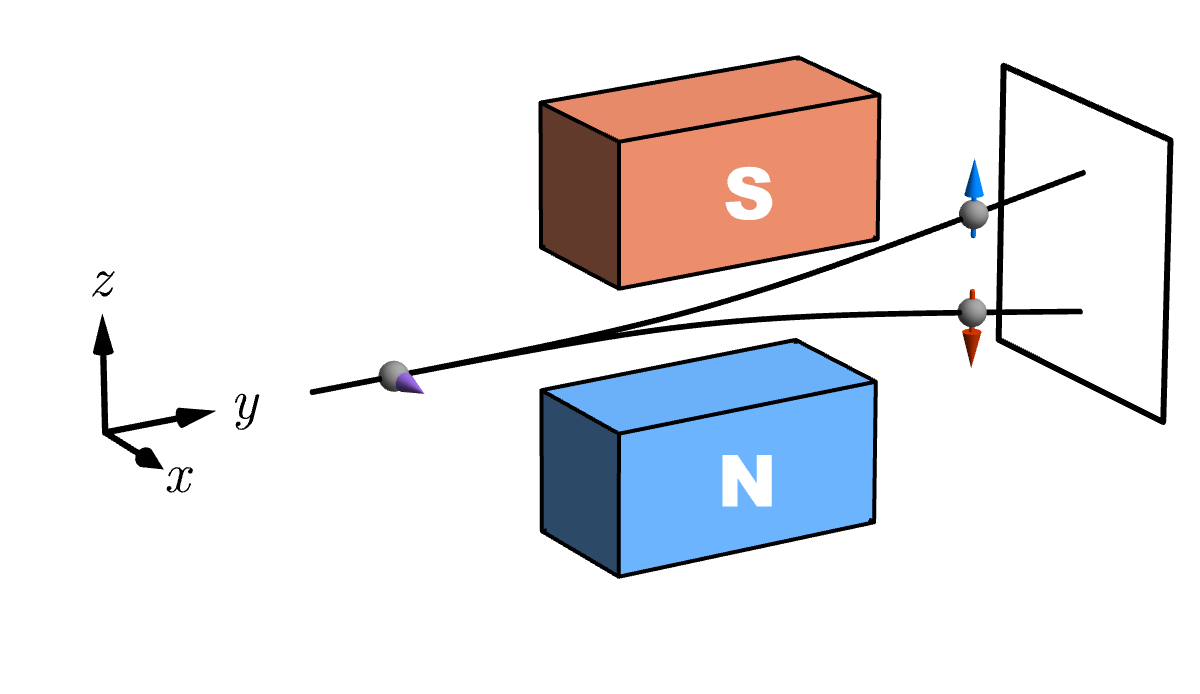
../images/1-2-1-stern_gerlach.png — Fig. 2 Stern-Gerlach setup: an inhomogeneous magnetic field spatially separates beams by spin projection, enabling state preparation and measurement.#

Experiment 1: Z-Z-Z (Sequential Stern-Gerlach)

Assume we start with 1000 atoms in an unpolarized (maximally mixed) ensemble \(\rho_0 = \tfrac{1}{2}\vert\uparrow\rangle\langle\uparrow\vert + \tfrac{1}{2}\vert\downarrow\rangle\langle\downarrow\vert\).

Step	Observable	Incoming state	Outcomes (Born rule)	Selection	Atoms (approx.)	Outgoing state
1 (prep)	\(\hat{\sigma}^z\)	depolarized ensemble	\(P(m)=\begin{cases}\tfrac{1}{2}, & m=+1\\ \tfrac{1}{2}, & m=-1\end{cases}\)	Keep \(+1\) branch	500	\(\vert\uparrow\rangle\)
2	\(\hat{\sigma}^z\)	\(\vert\uparrow\rangle\)	\(P(m)=\begin{cases}1, & m=+1\\ 0, & m=-1\end{cases}\)	Keep \(+1\) branch	500	\(\vert\uparrow\rangle\)
3	\(\hat{\sigma}^z\)	\(\vert\uparrow\rangle\)	\(P(m)=\begin{cases}1, & m=+1\\ 0, & m=-1\end{cases}\)	Keep \(+1\) branch	500	\(\vert\uparrow\rangle\)

What Experiment 1 teaches us:

The measurement outcome is binary: the beam always splits into exactly two components, never a continuum.
The first apparatus doubles as a state-preparation device: filtering one branch by post-selection prepares a definite pure state.
Repeatability: measuring the same observable twice in a row always confirms the first result — the outcome is reproducible, suggesting the existence of an underlying physical reality that persists between measurements.

Experiment 2: Z-X-Z (Incompatible Measurements)

Again start with 1000 atoms in the same depolarized ensemble.

Step	Observable	Incoming state	Outcomes (Born rule)	Selection	Atoms (approx.)	Outgoing state
1 (prep)	\(\hat{\sigma}^z\)	depolarized ensemble	\(P(m)=\begin{cases}\tfrac{1}{2}, & m=+1\\ \tfrac{1}{2}, & m=-1\end{cases}\)	Keep \(+1\) branch	500	\(\vert\uparrow\rangle\)
2	\(\hat{\sigma}^x\)	\(\vert\uparrow\rangle\)	\(P(m)=\begin{cases}\tfrac{1}{2}, & m=+1\\ \tfrac{1}{2}, & m=-1\end{cases}\)	Keep \(+1\) branch	250	\(\vert\rightarrow\rangle\)
3	\(\hat{\sigma}^z\)	\(\vert\rightarrow\rangle\)	\(P(m)=\begin{cases}\tfrac{1}{2}, & m=+1\\ \tfrac{1}{2}, & m=-1\end{cases}\)	Keep \(-1\) branch	125	\(\vert\downarrow\rangle\)

What Experiment 2 teaches us:

The intermediate X measurement washes out the previously definite Z outcome — the final Z result is now random again.
Measurement is invasive: it is not a passive readout of a pre-existing value, but an active intervention that can alter the state.
Non-commuting measurements change reality — inserting \(\hat{\sigma}^x\) between two \(\hat{\sigma}^z\) measurements destroys the Z-definiteness that Experiment 1 established.

Building the Mathematical Model#

Goal: Find a formula \(P(m \vert \psi, \hat{O})\) for the probability of obtaining outcome \(m\) when measuring observable \(\hat{O}\) on state \(\vert\psi\rangle\).

Positivity constraint: Since \(P(m \vert \psi, \hat{O}) \geq 0\) for all states \(\vert\psi\rangle\), we need a mathematical object that is guaranteed non-negative for any input state. A natural choice is to model \(P\) as the expectation value of some operator \(\hat{P}_{O=m}\):

\[ P(m \vert \psi, \hat{O}) = \langle \psi \vert \hat{P}_{O=m} \vert \psi \rangle \]

This is automatically non-negative if \(\hat{P}_{O=m}\) is positive semi-definite (PSD).

Positive Semi-Definite (PSD) Operator

An operator \(\hat{A}\) is positive semi-definite if \(\langle \psi \vert \hat{A} \vert \psi \rangle \geq 0\) for all states \(\vert\psi\rangle\). Equivalently, all eigenvalues of \(\hat{A}\) are \(\geq 0\).

Pinning down the operator: The SG experiments (Z-Z-Z) showed that repeatedly measuring the same observable on an eigenstate \(\vert O{=}m\rangle\) always returns \(m\). This means:

\[ P(m \vert O{=}m, \hat{O}) = 1, \quad P(m' \vert O{=}m, \hat{O}) = 0 \text{ for } m' \neq m \]

What PSD operator satisfies this? The projection operator \(\hat{P}_{O=m} = \vert O{=}m\rangle\langle O{=}m\vert\).

Verification: Projector Gives the Right Probabilities

For eigenstate \(\vert\psi\rangle = \vert O{=}m\rangle\):

\[ P(m \vert O{=}m, \hat{O}) = \langle O{=}m \vert \hat{P}_{O=m} \vert O{=}m \rangle = \langle O{=}m \vert O{=}m\rangle \langle O{=}m \vert O{=}m \rangle = 1 \quad \checkmark \]

For a different eigenstate \(\vert\psi\rangle = \vert O{=}m'\rangle\) with \(m' \neq m\):

\[ P(m \vert O{=}m', \hat{O}) = \langle O{=}m' \vert \hat{P}_{O=m} \vert O{=}m' \rangle = \vert\langle O{=}m \vert O{=}m' \rangle\vert^2 = 0 \quad \checkmark \]

(using orthogonality of eigenstates).

For a general superposition \(\vert\psi\rangle = c_1 \vert O{=}m_1\rangle + c_2 \vert O{=}m_2\rangle\) with \(\vert c_1\vert^2 + \vert c_2\vert^2 = 1\):

\[ P(m_1 \vert \psi, \hat{O}) = \vert c_1\vert^2, \quad P(m_2 \vert \psi, \hat{O}) = \vert c_2\vert^2, \quad \text{sum} = 1 \quad \checkmark \]

This gives us the Born rule: the probability of outcome \(m\) is the squared overlap with the corresponding eigenstate,

\[ P(m \vert \psi, \hat{O}) = \langle \psi \vert \hat{P}_{O=m} \vert \psi \rangle = \vert\langle O{=}m \vert \psi \rangle\vert^2 \]

The Measurement Postulate#

The Measurement Postulate

Axiom 1 (Possible Outcomes): When measuring observable \(\hat{O}\), the only possible outcomes are its eigenvalues \(m\).

Axiom 2 (Born Rule): The probability of obtaining outcome \(m\) from state \(\vert\psi\rangle\) is

\[ P(m | \psi, \hat{O}) = \vert \langle O=m \vert \psi \rangle\vert^2 \]

where \(\vert O=m\rangle\) is the (normalized) eigenstate corresponding to eigenvalue \(m\).

Axiom 3 (State Collapse): Immediately after obtaining outcome \(m\), the state collapses to the corresponding eigenstate:

\[ \vert\psi\rangle \xrightarrow[\text{measure } \hat{O}]{\text{outcome } m} \vert O=m\rangle \]

Interpretation of collapse: After the measurement, the system is no longer in a superposition. All information about the pre-measurement state is lost (unless we knew the outcome beforehand). This is irreversible and fundamental to quantum mechanics.

Explaining the Stern-Gerlach Experiments#

The process tables above can be summarized algebraically:

\(\vert\uparrow\rangle\) is an eigenstate of \(\hat{\sigma}^z\), so repeated Z-measurement is deterministic.
Decomposed to \(\hat{\sigma}^x\)-basis:

\[ \vert\uparrow\rangle = \frac{1}{\sqrt{2}}\left(\vert\rightarrow\rangle + \vert\leftarrow\rangle\right) \]

On Z-basis state \(\vert\uparrow\rangle\), X-measurement outcomes 50-50.

Symmetry argument: \(\vert\rightarrow\rangle\) and \(\vert\leftarrow\rangle\) looks symmetric from \(\vert\uparrow\rangle\) perspective, so they must have identical probability to be observed.
Select \(\vert\rightarrow\rangle\), decompose to \(\hat{\sigma}^z\)-basis again:

\[ \vert\rightarrow\rangle = \frac{1}{\sqrt{2}}\left(\vert\uparrow\rangle + \vert\downarrow\rangle\right) \]

So selecting one X branch (e.g. \(\vert\rightarrow\rangle\)) makes the final Z outcomes 50-50. This is quantum complementarity: the intermediate X measurement erases prior Z-definiteness.

Discussion: simultaneous spin definiteness

Why can’t we prepare atoms to have definite spin-up in both z and x directions simultaneously?

The eigenstates of \(\hat{\sigma}^z\) are \(\{\vert\uparrow\rangle, \vert\downarrow\rangle\}\). The eigenstates of \(\hat{\sigma}^x\) are \(\{\vert\rightarrow\rangle, \vert\leftarrow\rangle\}\). These bases are orthogonal (perpendicular in Hilbert space). A state that is an eigenstate of one operator is a superposition in the other operator’s basis.

This is not a limitation of experiment—it is built into the structure of quantum mechanics. Non-commuting observables cannot be simultaneously definite.

Poll: Measurement collapse

A qubit in state \(\vert\psi\rangle = \frac{1}{\sqrt{2}}(\vert 0\rangle + \vert 1\rangle)\) is measured and gives outcome 0. Immediately afterward, you measure again. What happens?

(A) You get 0 again with 50% probability (independent measurements).

(B) You definitely get 0 (measurement collapses the state).

(D) The result depends on how quickly you measure the second time.

Summary#

Measurement is fundamental: It yields a definite outcome (an eigenvalue), irreversibly collapses the state to the corresponding eigenstate, and follows the Born rule: \(P(m) = |\langle O=m|\psi\rangle|^2\).
The measurement postulate formalizes this via three axioms: outcomes are eigenvalues, probabilities follow Born rule, and collapse is instantaneous and irreversible.
Stern-Gerlach experiments directly demonstrate collapse: repeated measurement is deterministic (Z-Z-Z), but incompatible measurements (Z-X-Z) erase prior definiteness, showing measurement is invasive, not passive readout.
Complementarity: Non-commuting observables cannot be simultaneously definite; inserting a measurement in an incompatible basis destroys prior measurement information.

Homework#

1. Measurement probabilities and collapse. A qubit is in the state \(\vert\psi\rangle = \dfrac{2\vert 0\rangle + \sqrt{5}\vert 1\rangle}{3}\). Measure \(\hat{Z}\).

(a) Compute \(P(+1)\) and \(P(-1)\) from the Born rule. Verify the probabilities sum to \(1\).

(b) Write the state immediately after obtaining outcome \(-1\), and explain in one sentence why the pre-measurement amplitudes \(c_0, c_1\) play no further role in subsequent dynamics.

2. Sequential measurements and filters. Start with the state \(\vert+\rangle = \tfrac{1}{\sqrt{2}}(\vert 0\rangle + \vert 1\rangle)\).

(a) Measure \(\hat{Z}\): find the probabilities and the post-measurement state for each outcome.

(b) Immediately after measuring \(\hat{Z}\) and obtaining outcome \(+1\), measure \(\hat{X}\). What are the outcome probabilities now?

(c) Compare with measuring \(\hat{X}\) directly on the original \(\vert+\rangle\). Explain in one sentence why the two procedures give different \(\hat{X}\) statistics — using the language of the lecture’s Z-X-Z experiment.

3. Measurement of a non-Pauli observable. Consider the Hermitian observable \(\hat{H} = \omega\,\hat{X} + \Delta\,\hat{Z}\) from 1.1.3 Problem 1, with \(\omega, \Delta > 0\). Its eigenvalues are \(E_\pm = \pm\Omega\) where \(\Omega = \sqrt{\omega^2 + \Delta^2}\), and its eigenstates parametrise the Bloch axis with mixing angle \(\theta_0\) defined by \(\tan\theta_0 = \omega/\Delta\):

\[ \vert E_+\rangle = \cos(\theta_0/2)\,\vert 0\rangle + \sin(\theta_0/2)\,\vert 1\rangle, \qquad \vert E_-\rangle = \sin(\theta_0/2)\,\vert 0\rangle - \cos(\theta_0/2)\,\vert 1\rangle. \]

A system is prepared in \(\vert 0\rangle\) and one measures \(\hat H\).

(a) List the possible outcomes.

(b) Compute the probability of each outcome. Express the answer as a function of \(\Delta/\Omega\).

(d) Compute \(\langle\hat H\rangle\) on the prepared state \(\vert 0\rangle\) in two ways — directly from \(\langle 0\vert\hat H\vert 0\rangle\), and via the spectral sum \(\sum_m m\,P(m)\) — and verify they agree.

4. State inference from measurement frequencies. An unknown qubit state \(\vert\psi\rangle\) is prepared on many identical copies. Measuring the three Pauli observables on these copies yields the relative frequencies

\[\begin{split} \begin{array}{l|cc} \text{basis} & f(+1) & f(-1) \\ \hline \hat Z & 0.70 & 0.30 \\ \hat X & 0.96 & 0.04 \\ \hat Y & 0.50 & 0.50 \\ \end{array} \end{split}\]

In the limit of infinitely many copies these frequencies equal the Born-rule probabilities. Assume this limit and reconstruct \(\vert\psi\rangle\).

(a) Compute the Bloch vector \(\boldsymbol n = (\langle\hat X\rangle, \langle\hat Y\rangle, \langle\hat Z\rangle)\). (Recall \(\langle\hat O\rangle = P(+1) - P(-1)\) for Pauli \(\hat O\).)

(b) Verify \(\vert\boldsymbol n\vert = 1\), consistent with the assumption that the source produces a pure state.

\[ \vert\psi\rangle = \cos(\theta/2)\,\vert 0\rangle + \mathrm{e}^{\mathrm{i}\varphi}\,\sin(\theta/2)\,\vert 1\rangle. \]

(d) Two of the three measurement bases give relative frequencies close to \(0\) or \(1\), while the third gives an equal split. Identify which Bloch-sphere axis the state’s Bloch vector lies closest to, and explain in one sentence why a measurement along that axis would have made the inference unambiguous from a single basis.

5. Phase erasure by complementary measurement. A qubit is prepared in the general Bloch state \(\vert\psi\rangle = \cos(\theta/2)\vert 0\rangle + \mathrm{e}^{\mathrm{i}\varphi}\sin(\theta/2)\vert 1\rangle\). Consider two scenarios for measuring \(\hat X\):

Scenario A (direct): Measure \(\hat X\) directly on \(\vert\psi\rangle\).
Scenario B (preceded by \(\hat Z\)): First measure \(\hat Z\) (record the outcome but do not post-select); the system collapses to one of \(\vert 0\rangle\) or \(\vert 1\rangle\). Then measure \(\hat X\) on the collapsed state.

(a) Compute \(P_A(\hat X = +1)\) for Scenario A. Express the answer in terms of \(\theta\) and \(\varphi\).

(b) Compute \(P_B(\hat X = +1)\) for Scenario B, marginalising over the (unobserved) Z outcome:

\[ P_B(\hat X = +1) = \sum_{m_1 = \pm 1} P(\hat Z = m_1)\,P(\hat X = +1\,\vert\,\text{post-}\hat Z\text{ state}). \]

Show that \(P_B(\hat X = +1) = 1/2\) — independent of \(\theta\) and \(\varphi\).

(c) Subtract: the difference between the two scenarios is \(P_A - P_B = \tfrac{1}{2}\sin\theta\cos\varphi\). Identify which part of the initial state’s Bloch vector controls this difference, and explain in one sentence why the intervening \(\hat Z\) measurement erased this contribution.

(d) For which initial Bloch directions is the erasure ineffective (\(P_A = P_B\))? Identify those locations on the Bloch sphere and explain physically why the \(\hat Z\) measurement leaves them untouched.

6. Quantum interference. Two qubit states differ only by a relative phase:

\[ \vert\psi_1\rangle = \tfrac{1}{\sqrt{2}}(\vert 0\rangle + \vert 1\rangle), \qquad \vert\psi_2\rangle = \tfrac{1}{\sqrt{2}}(\vert 0\rangle + \mathrm{e}^{\mathrm{i}\varphi}\vert 1\rangle), \quad \varphi\in\mathbb R. \]

(a) Show that \(\hat Z\) measurements on \(\vert\psi_1\rangle\) and \(\vert\psi_2\rangle\) produce identical outcome probabilities.

(b) Compute \(P(+1)\) for \(\hat X\) measured on \(\vert\psi_2\rangle\) as a function of \(\varphi\).

(c) Explain in one sentence why the relative phase is invisible to \(\hat Z\) but visible to \(\hat X\), in terms of how each measurement combines the amplitudes \(c_0\) and \(c_1\).

7. Filter vs measurement misconception. Consider a Stern-Gerlach setup:

\[ \hat{Z} \to \text{(filter }+1\text{)} \to \hat{X} \to \text{(filter }-1\text{)} \to \hat{Z}. \]

Atoms enter in state \(\vert 0\rangle\). The first apparatus measures \(\hat Z\) and keeps only the \(+1\) branch; the second measures \(\hat X\) and keeps only the \(-1\) branch; the third measures \(\hat Z\) but has no filter — every atom that reaches it is measured and recorded.

(a) Compute the surviving fraction of the original beam after each apparatus.

(b) What is the final state of an atom that makes it all the way through? Give both possible outcomes of the final \(\hat Z\) measurement and their conditional probabilities.

(c) A naive analysis multiplies the Born-rule outcome probabilities at every stage, obtaining \(1 \times \tfrac{1}{2} \times \tfrac{1}{2} = \tfrac{1}{4}\) for the surviving fraction. Identify the error in this analysis, and explain in one sentence the difference between a filter (post-selects a branch, discarding the rest) and a measurement (records the outcome on every atom but discards none).