4.2.2 Aharonov-Bohm Effect#
Prompts
Why does an electron acquire a quantum phase shift after passing around a solenoid even though it travels entirely in a \(\boldsymbol{B}=0\) region? Where does the phase come from if the Lorentz force vanishes everywhere on the path?
What is the Aharonov-Bohm phase \(\Delta\Phi_{\mathrm{AB}} = q\Phi/\hbar\) telling us about the relationship between \(\boldsymbol{A}\) and \(\boldsymbol{B}\)? Why is the closed-loop integral \(\oint\boldsymbol{A}\cdot\mathrm{d}\boldsymbol{l}\) gauge-invariant while \(\boldsymbol{A}\) itself is not?
How does the AB effect realise the closed-loop Berry phase in real space, with the particle’s position as the parameter and \(q\boldsymbol{A}/\hbar\) as the gauge connection?
Why does the AB phase depend only on the winding number of the path around the solenoid, not on its shape or speed? What does the multiply-connected geometry of the field-free region have to do with this?
How did Tonomura’s electron-holography experiment on toroidal magnets confirm the Aharonov-Bohm effect? Why is a torus with its flux fully confined by a superconducting shield a cleaner test than an infinite solenoid — what classical objection does the confined geometry rule out?
Why is the AB effect taken as evidence that the vector potential is physical in quantum mechanics, even though no measurement can determine \(\boldsymbol{A}\) pointwise?
Lecture Notes#
Overview#
The Aharonov-Bohm (AB) effect demonstrates that a charged particle’s quantum phase depends on the electromagnetic vector potential \(\boldsymbol{A}\), even when its trajectory stays entirely in a region where the magnetic field vanishes. It is the canonical real-space realisation of the closed-loop Berry phase developed in 4.2.1 Berry Phase: the parameter is the particle’s position, the gauge connection on that parameter space is \(q\boldsymbol{A}/\hbar\), and the holonomy around any loop that encircles the solenoid is the gauge-invariant Berry phase.
Setup: solenoid in a multiply-connected region#
A long solenoid carries a uniform magnetic field \(\boldsymbol{B}\) confined to its interior; outside the solenoid \(\boldsymbol{B} = 0\). An electron beam is split into two paths \(\mathcal{C}_\text{upper}\) and \(\mathcal{C}_\text{lower}\) that pass around opposite sides of the solenoid and recombine on a screen.
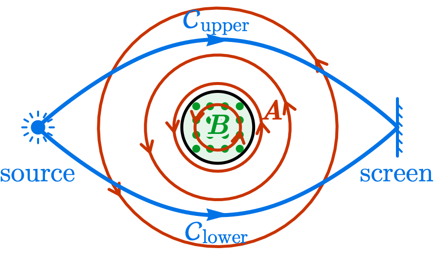
Fig. 18 Schematic AB setup: paths \(\mathcal{C}_\text{upper}\) and \(\mathcal{C}_\text{lower}\) enclose the solenoid; \(\boldsymbol{B}\) is confined inside, but \(\boldsymbol{A}\) extends outside, so the relative phase depends on \(\oint\boldsymbol{A}\cdot\mathrm{d}\boldsymbol{l}\).#
In the field-free region outside the solenoid the vector potential is not zero. Its curl vanishes locally, but the region is multiply connected — any loop enclosing the solenoid cannot be contracted to a point without crossing the field region — so \(\boldsymbol{A}\) cannot be written as the gradient of a single-valued function on the whole field-free region. By Stokes’ theorem, the circulation of \(\boldsymbol{A}\) around any loop encircling the solenoid equals the magnetic flux through any surface that spans the loop,
regardless of the choice of \(\mathcal{S}\) — the flux is the same through any cap, because \(\nabla\cdot\boldsymbol{B} = 0\) guarantees that no field lines are lost in between.
Classically, the electron experiences no Lorentz force along either path (\(\boldsymbol{F} = q\boldsymbol{v}\times\boldsymbol{B} = 0\)), so the two paths should produce identical interference fringes. The quantum-mechanical result is that the fringe pattern shifts when the flux through the solenoid is changed.
AB phase from two-path interference#
In any simply connected sub-region where \(\boldsymbol{B}=0\), the local gauge freedom of 4.1.3 Gauge Invariance allows one to gauge \(\boldsymbol{A}\) away along a path. Reverting the local gauge transformation reveals that, along a path \(\mathcal{C}\), the wavefunction picks up a path-dependent phase factor relative to its \(\boldsymbol{A}=0\) counterpart.
Derivation: Single-Path Phase from Local Gauge Transformation
Setup. In any simply connected sub-region where \(\boldsymbol{B} = \nabla\times\boldsymbol{A} = 0\), the vector potential is curl-free and can be written as a pure gradient. Along a chosen path \(\mathcal{C}\) from \(\boldsymbol{x}_0\) to \(\boldsymbol{x}\), define the gauge function
Path-independence of line integrals of a curl-free field within the simply connected region (Stokes’ theorem with \(\nabla\times\boldsymbol{A}=0\)) makes \(\alpha\) a well-defined function of the endpoint, and the fundamental theorem of calculus gives \(\nabla\alpha = -\boldsymbol{A}\).
Apply the local gauge transformation from 4.1.3 Gauge Invariance with this \(\alpha\):
The transformed wavefunction \(\tilde\psi(\boldsymbol{x}) \equiv \mathrm{e}^{\mathrm{i}q\alpha(\boldsymbol{x})/\hbar}\psi(\boldsymbol{x})\) satisfies the Schrödinger equation in the \(\boldsymbol{A}=0\) gauge along \(\mathcal{C}\) and therefore carries no path-dependent EM phase.
Invert the transformation to read off the path-dependent phase of the original \(\psi\):
so along \(\mathcal{C}\) the wavefunction differs from its \(\boldsymbol{A}=0\) counterpart by the path-dependent phase
Around the solenoid the field-free region is multiply connected, so the simply connected construction breaks: no global \(\boldsymbol{A}=0\) gauge exists, and the two interfering paths’ phases need not agree.
The two interfering paths’ single-path phases differ:
Reversing the orientation of the lower path joins the two segments into a single closed contour \(\mathcal{C} = \mathcal{C}_\text{upper} - \mathcal{C}_\text{lower}\) that encircles the solenoid:
Aharonov-Bohm Phase
A charged particle’s two-path interference around a solenoid picks up a relative phase
where \(\Phi\) is the magnetic flux enclosed by the loop. Even though the trajectory itself stays in \(\boldsymbol{B} = 0\), any surface \(\mathcal{S}\) spanning \(\mathcal{C}\) must cut the solenoid and capture the full flux \(\Phi\) inside.
Periodicity. The AB phase enters the interference intensity through \(\mathrm{e}^{\mathrm{i}\Delta\Phi_{\mathrm{AB}}}\), so the pattern is periodic in \(\Phi\) with natural period
For an electron (\(q=e\)), \(\Phi_0 = h/e \approx 4.14\times 10^{-15}\,\text{Wb}\). This sets the natural period of the AB phase; it is set by the carrier charge and does not by itself quantize \(\Phi\), which remains a continuous parameter. A genuine quantization of \(\Phi\) requires a macroscopic single-valued wavefunction, taken up in 4.2.3 Flux Ring.
Topology and gauge invariance#
Two features distinguish the AB phase from a generic line integral and make it a physical observable.
Winding number, not shape. The AB phase depends only on whether the closed contour \(\mathcal{C}\) encircles the solenoid, not on its detailed shape. Smoothly deforming \(\mathcal{C}\) inside the \(\boldsymbol{B} = 0\) region leaves \(\oint_\mathcal{C}\boldsymbol{A}\cdot\mathrm{d}\boldsymbol{l}\) unchanged; pushing \(\mathcal{C}\) across the solenoid changes its winding number by \(\pm 1\) and shifts the phase by \(\pm q\Phi/\hbar\). The AB phase is a function of the path’s homotopy class in the multiply-connected field-free region — a topological invariant, not a geometric quantity.
Gauge invariance of the closed-loop integral. Under \(\boldsymbol{A} \to \boldsymbol{A} + \nabla\alpha\), an open-path integral shifts by the boundary values of \(\alpha\), but the closed-loop integral is invariant: \(\oint\nabla\alpha\cdot\mathrm{d}\boldsymbol{l} = 0\) for any single-valued \(\alpha\). This is the same open-vs-closed dichotomy as the EM holonomy of 4.1.3 Gauge Invariance and the Berry phase of 4.2.1 Berry Phase.
Closed-Loop Holonomy of A
The physically observable content of the vector potential in quantum mechanics is its closed-loop holonomy \(\oint\boldsymbol{A}\cdot\mathrm{d}\boldsymbol{l}\), not \(\boldsymbol{A}\) at any individual point. Pointwise \(\boldsymbol{A}\) is gauge-dependent and unobservable; any single-valued gauge transformation \(\boldsymbol{A}\to\boldsymbol{A}+\nabla\alpha\) leaves the closed-loop integral unchanged. In a multiply-connected \(\boldsymbol{B} = 0\) region, no single-valued gauge transformation can make the holonomy vanish, and the AB phase \(\oint\boldsymbol{A}\cdot\mathrm{d}\boldsymbol{l} = \Phi\) is a genuine physical observable of \(\boldsymbol{A}\) — one not visible in any local measurement of \(\boldsymbol{E}\) or \(\boldsymbol{B}\).
Discussion: Is A More Fundamental Than B?
In classical mechanics, a particle’s trajectory depends only on \(\boldsymbol{E}\) and \(\boldsymbol{B}\) through the Lorentz force; the vector potential \(\boldsymbol{A}\) does not appear. In quantum mechanics, \(\boldsymbol{A}\) enters the Schrödinger equation via minimal coupling, making it observable in gauge-invariant combinations. Is the AB effect a sign that quantum mechanics is “deeper” than classical mechanics, or simply that we must describe particles by wavefunctions rather than trajectories? Are \(\boldsymbol{A}\) and \(\boldsymbol{B}\) on equal footing as physical fields, or is one more fundamental?
Experimental confirmation#
The classical objection “but the solenoid has stray fringing fields that deflect the electron classically” was definitively ruled out by Tonomura et al. (1986), who used electron holography on toroidal magnets in which the magnetic field was fully confined inside the donut by a superconducting shield. With no \(\boldsymbol{B}\) leakage anywhere outside the toroid, the interference pattern still shifted in exact accord with \(\Delta\Phi_{\mathrm{AB}} = q\Phi/\hbar\) as the trapped flux was varied.
Poll: quantum phase from the vector potential
A charged particle traveling in a region where \(\boldsymbol{B} = 0\) still acquires a phase shift \(\Delta\Phi_{\mathrm{AB}} = q\Phi/\hbar\) between two paths enclosing a solenoid. Which statement best explains why?
(A) The vector potential is the fundamental physical quantity; the magnetic field is a derived auxiliary with no direct physical meaning.
(B) The minimal-coupling Schrödinger equation contains \(\hat{\boldsymbol{p}} - q\boldsymbol{A}\), so the wavefunction’s phase responds directly to \(\boldsymbol{A}\); the gauge-invariant observable is the closed-loop holonomy \(\oint\boldsymbol{A}\cdot\mathrm{d}\boldsymbol{l}\).
(C) The electron must briefly tunnel into the solenoid where \(\boldsymbol{B}\ne 0\), so the phase comes from rare excursions into the field region.
(D) The Bohr-Sommerfeld quantization condition forces the enclosed flux to be quantized, producing the phase shift.
Summary#
The Aharonov-Bohm phase \(\Delta\Phi_{\mathrm{AB}} = q\Phi/\hbar\) is the closed-loop Berry phase of a charged particle whose path encircles a solenoid in a region where \(\boldsymbol{B} = 0\) everywhere on the trajectory.
It enters interference through \(\mathrm{e}^{\mathrm{i}\Delta\Phi_{\mathrm{AB}}}\), so the pattern is periodic in the enclosed flux with natural period \(\Phi_0 = h/q\) set by the carrier charge.
The phase is topological: it depends only on the winding number of the loop around the solenoid, not on its shape or traversal speed.
The closed-loop integral \(\oint\boldsymbol{A}\cdot\mathrm{d}\boldsymbol{l}\) is gauge-invariant even though \(\boldsymbol{A}\) itself is not; an open-path integral on a single arm is gauge-dependent and unobservable.
In quantum mechanics the gauge-invariant content of \(\boldsymbol{A}\) — its closed-loop holonomies — is physically real in multiply-connected \(\boldsymbol{B} = 0\) regions, as confirmed experimentally by Tonomura’s toroidal-magnet measurements.
See Also
4.2.1 Berry Phase: parent concept; AB is the closed-loop Berry phase with parameter the particle position and connection \(q\boldsymbol{A}/\hbar\).
4.1.3 Gauge Invariance: the open-vs-closed dichotomy in real space; the EM holonomy that the AB phase realises.
4.2.3 Flux Ring: a concrete particle-on-a-ring model where the AB phase enters the energy spectrum; persistent currents, flux quantization in superconductors, and SQUIDs.
Homework#
1. Invisible solenoid. An electron double-slit experiment is performed around an extremely thin solenoid carrying flux \(\Phi\). The electron never enters the solenoid, so \(\boldsymbol{B} = 0\) everywhere on its path.
(a) Show that the fringe pattern shifts by \(\Delta\Phi_{\mathrm{AB}}/(2\pi)\) fringes, where \(\Delta\Phi_{\mathrm{AB}} = e\Phi/\hbar\). For \(\Phi = h/(2e)\), how many fringes does the pattern shift?
(b) A skeptic says: “The solenoid has fringing fields that leak out and deflect the electron classically.” Design an idealised experiment that rules out this objection. (Hint: what if the solenoid is enclosed in a superconducting shield?)
(c) If \(\Phi\) is increased continuously from \(0\) to \(\Phi_0 = h/e\), the fringe pattern returns to its original position. Explain why the interference intensity is periodic in flux with period \(\Phi_0\), while \(\Phi\) itself remains a continuous parameter.
2. Which path matters. Two paths \(\mathcal{C}_1\) and \(\mathcal{C}_2\) connect points \(A\) and \(B\) in a region where \(\boldsymbol{B} = 0\).
(a) Show that the phase difference \(\Delta\Phi_{\mathrm{AB}} = \Phi_{\mathrm{path}}[\mathcal{C}_1] - \Phi_{\mathrm{path}}[\mathcal{C}_2]\) depends only on whether the combined loop \(\mathcal{C}_1 - \mathcal{C}_2\) encloses flux, not on the shapes of the individual paths.
(b) A third path \(\mathcal{C}_3\) also connects \(A\) to \(B\) but winds twice around the solenoid. What is \(\Phi_{\mathrm{path}}[\mathcal{C}_3] - \Phi_{\mathrm{path}}[\mathcal{C}_1]\) in terms of \(\Phi\)?
(c) Classify all paths from \(A\) to \(B\) by their winding number around the solenoid. How does this classification reflect the multiply-connected topology of the field-free region?
3. Gauge dependence of single paths. Under a gauge transformation \(\boldsymbol{A} \to \boldsymbol{A} + \nabla\alpha\), the phase accumulated along a single path \(\mathcal{C}\) from \(P\) to \(Q\) changes.
(a) Show that \(\Phi_{\mathrm{path}}'[\mathcal{C}] = \Phi_{\mathrm{path}}[\mathcal{C}] + (q/\hbar)[\alpha(Q) - \alpha(P)]\).
(b) Explain why this makes the single-path phase unobservable, but the relative phase between two paths sharing endpoints remains gauge-invariant.
(c) One might claim: “I can always choose a gauge in which \(\boldsymbol{A} = 0\) outside the solenoid, so there is no AB effect.” Find the flaw. Can \(\boldsymbol{A}\) be set to zero everywhere in a multiply-connected region with nonzero enclosed flux by a single-valued gauge function?
4. Surface independence. Stokes’ theorem turns the AB loop integral into a magnetic flux through any surface \(\mathcal{S}\) that spans the loop \(\mathcal{C}\). The result should not depend on which surface one chooses.
(a) Let \(\mathcal{S}_1\) and \(\mathcal{S}_2\) be two oriented surfaces that both span the same loop \(\mathcal{C}\), together enclosing a volume \(V\) with \(\mathcal{S}_1 - \mathcal{S}_2 = \partial V\). Use the divergence theorem to show
(b) Maxwell’s equation \(\nabla\cdot\boldsymbol{B} = 0\) forces the two flux integrals to agree. Conclude that the AB phase is well-defined independently of the surface used in Stokes’ theorem.
(c) Suppose a magnetic monopole of charge \(g\) sat between \(\mathcal{S}_1\) and \(\mathcal{S}_2\), so that \(\nabla\cdot\boldsymbol{B} = \mu_0\rho_m\) with a delta-function source. Compute the discrepancy in terms of \(g\) and explain why the AB phase would be ambiguous absent the Dirac quantization condition introduced in 4.4.2 Dirac Monopole.
5. AB phase as Berry phase. The AB phase is the closed-loop Berry phase of a charged particle whose parameter happens to be its own position.
(a) Identify the parameter space: as the electron’s position \(\boldsymbol{r}\) winds around the solenoid, what plays the role of the parameter \(\boldsymbol{R}\) in the Berry-phase formalism of 4.2.1 Berry Phase?
(b) Show that, for a wavefunction \(\psi(\boldsymbol{r}) = \mathrm{e}^{\mathrm{i}q\int^{\boldsymbol{r}}\boldsymbol{A}\cdot\mathrm{d}\boldsymbol{l}'/\hbar}\tilde\psi(\boldsymbol{r})\) with \(\tilde\psi\) the gauge-rotated background state, the Berry connection \(\boldsymbol{A}_\text{Berry} = \mathrm{i}\langle\psi(\boldsymbol{r})\vert\nabla_{\boldsymbol{r}}\vert\psi(\boldsymbol{r})\rangle\) reduces to \((q/\hbar)\boldsymbol{A}(\boldsymbol{r})\).
(c) Verify that the closed-loop Berry phase is \(\oint\boldsymbol{A}_\text{Berry}\cdot\mathrm{d}\boldsymbol{r} = q\Phi/\hbar\) and that this answer is independent of the gauge chosen for \(\boldsymbol{A}\).
6. Electric Aharonov-Bohm. A charged particle passes through a region of zero electric field, but the scalar potential \(\phi\) is nonzero and time-dependent.
(a) Two electron wavepackets travel through two tubes at different electrostatic potentials \(V_1\) and \(V_2\) for a time \(T\), with \(\boldsymbol{E} = 0\) everywhere the electrons travel. Show that the relative phase is \(\Delta\Phi = eT(V_1 - V_2)/\hbar\).
(b) Explain why this is analogous to the magnetic AB effect: the potential produces a measurable phase even though no force acts on the particle.
(c) Is the electric AB effect topological in the same sense as the magnetic one? What role does the multiply-connected geometry play in each case?
7. Toroidal magnet. Tonomura’s electron-holography test of the AB effect used a toroidal magnet (donut), not an infinite solenoid: the magnetic field is fully confined to the toroid’s interior, with zero field everywhere outside.
(a) An electron beam threads the central hole of the toroid; a reference beam bypasses it externally; the two recombine on a detector. Sketch the geometry, identify the loop \(\mathcal{C}\) that contributes to the AB phase, and show that \(\Delta\Phi_{\mathrm{AB}} = q\Phi_\text{inside}/\hbar\), where \(\Phi_\text{inside}\) is the flux through the toroid’s interior.
(b) Why is the toroidal geometry — with no field anywhere outside — a cleaner experimental test than the original infinite-solenoid geometry?
(c) Tonomura further coated the toroid with a superconducting shell to flux-trap the field inside. Using the Meissner effect (field expulsion by a superconductor), explain how this rules out the residual objection of stray fringing fields and makes the AB phase fully isolated from any local Lorentz force.